Loops¶

In this section we show how to exploit loops (for, while) within Python code snippets to define complicated geometries or project setups in a few number of script lines.

Loops within an embedded Python code block (cf. previous section Python Code Snippets) may extend over several blocks:

<?
for centerX in range(0, 10):
  keys['center'] = [centerX, 0.0]
  ?>

Circle {
  Radius = 0.5
  GlobalPosition = %(center)e
  ...
}

  <?  # closes for loop
?>

Here, a for-loop starts in line 2 within the first Python block. As a convention the <?, ?> starting and closing tags follow the Python indentation rules. Hence the for-loop is not closed in line 4, but in line 13 after a .jcm code block (lines 6-10).

Line 3 dynamically sets the value for key center, which serves as the circle’s center in line 8. This way, we have defined ten circles, equally spaced in $x$ -direction.

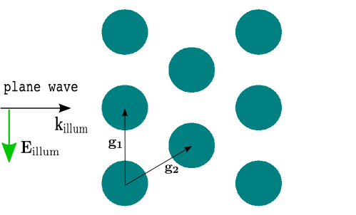
To see how this works in practice, we want to compute the light scattering off multiple rods aligned on a hexagonal lattice. Figure “Multiple rod geometry” shows the setup.

_images/phc_geometry.png — Multiple rod geometry¶

$\pvec{g}_1$ and $\pvec{g}_2$ are called grid vectors. For a hexagonal alignment we have

$\begin{eqnarray*} \pvec{g}_1 = a\cdot\left( \begin{array}{c} 0.0 \\ 1.0 \end{array} \right), \; \pvec{g}_2 = a\cdot \left( \begin{array}{c} \sin(60^\circ) \\ \cos(60^\circ) \end{array} \right), \end{eqnarray*}$

with a lattice parameter $a$ , which is passed as a further parameter in the driver script:

import jcmwave

# set problem parameter
keys = {
    'radius':  0.3,
    'a': 1.0,
    'n_rods': [3, 3],
    'n_air': 1.0,
    'n_glass': 1.52,
    'lambda_0': 0.550, # in um 
    'polarization': 45 # in degree
}

# run the project
results = jcmwave.solve('mie2D.jcmp', keys=keys)

# get scattering cross section
scattering_cross_section = results[1]['ElectromagneticFieldEnergyFlux'][0][0]
print ('\nscattering cross section: %.8g\n' % scattering_cross_section.real )

# plot exported cartesian grid within python
cfb = results[2]
amplitude = cfb['field'][0]
intensity = (amplitude.conj()*amplitude).sum(2).real 

from matplotlib.pyplot import *
pcolormesh(cfb['X'], cfb['Y'], intensity, shading='gouraud') 
axis('tight')
gca().set_aspect('equal')
gca().xaxis.major.formatter.set_powerlimits((-1, 0))
gca().yaxis.major.formatter.set_powerlimits((-1, 0))
show()

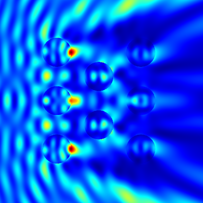
In line 7 we set the number of rods in $x$ - and $y$ - direction. Figure “Intensity” shows the computed intensity of the electric field.

_images/phc_intensity.png — Intensity¶

Pseudo-color intensity plot as produced by the driver `run.py`.

For this problem you again find a driver run_geo.py which only runs the mesh generation:

import jcmwave

# set geometry parameter
keys = {
    'radius':  0.3,
    'a': 1.0,
    'n_rods': [3, 3]
}

# generate mesh file only
jcmwave.geo('.', keys)

# open grid.jcm in JCMview
jcmwave.view('grid.jcm')

You can use this script to “play” with the geometry parameters and to watch how the geometry is updated.

In the following we want to discuss the updated layout file:

<?
# compute grid vectors for hexagonal grid

from math import sin, cos, pi
from numpy import array

gv1 = array([0.0, keys['a']])
gv2 = array([sin(60./180*pi), cos(60./180*pi)])*keys['a']

# compute computational domain enclosing all scatterer
maxX = (keys['n_rods'][0]-1)*gv2[0]
maxY = (keys['n_rods'][1]-1)*gv1[1]
    
keys['computational_domain_X'] = maxX+2*keys['radius']+2
keys['computational_domain_Y'] = maxY+2*keys['radius']+2     
?>


Layout2D {
  UnitOfLength = 1e-6

  MeshOptions {
    MaximumSideLength = 0.1
    CurvilinearDegree = 2
  }

  Objects {
    # Computational domain
    Parallelogram {
      DomainId = 1
      Width = %(computational_domain_X)e
      Height = %(computational_domain_Y)e
  
      # set transparent boundary conditions
      Boundary{
        Class = Transparent
      }
    }

<?
center_array = array([maxX/2, maxY/2])
for iX in range(0, keys['n_rods'][0]):
    col_start  = array([iX*gv2[0], (iX % 2)*gv2[1]])
    for iY in range(0, keys['n_rods'][1]-(iX % 2)):
        keys['center'] = col_start+iY*gv1-center_array 
        ?> 
    # Scatterer (rod)
    Circle {
      DomainId = 2
      Radius = %(radius)e
      GlobalPosition = %(center)e
    }
  
<? # closes for loops
?>
  }
}


 

The first Python block computes the grid vectors $\pvec{g}_1,$ $\pvec{g}_2$ (lines 7-8), and adapts the computational domain size to enclose all rods (lines 10-15). There, maxX and maxY are the dimensions of the array of rods in $x$ and $y$ .

The Python block from lines 38-46 defines two for loops over the number of rods in $x$ and $y$ . Line 43 sets the center of the current rod, which is used in line 51 in the enclosed .jcm block (center_array is used to shift the center of the array of rods to the origin). The for loops are closed in the last Python block (lines 56-57).