Parameter Reconstruction
In order to use the new JCMoptimizer, please follow the instructions in the JCMoptimizer documentation.
In this tutorial we briefly discuss how we can perform a parameter reconstruction using a Mueller matrix ellipsometry dataset. We use the same project files that were also used in the discussion on Mueller matrix ellipsometry in the EM tutorial example.
We assume that we have acquired a set of measurements from a Mueller matrix ellipsometry
experiment on a grating, that was performed for a series of different incident light
wavelengths  . These measurements are arranged in a target vector
 . As we control its construction we know which Mueller matrix element and wavelength contributes to which vector element.
We further assume that we can assign a measurement uncertainty
to each of the components in , we denote the measurement uncertainty vector
as
. As we control its construction we know which Mueller matrix element and wavelength contributes to which vector element.
We further assume that we can assign a measurement uncertainty
to each of the components in , we denote the measurement uncertainty vector
as  . Please note that the actual ordering of the components within the
vector is of no importance for the reconstruction.
. Please note that the actual ordering of the components within the
vector is of no importance for the reconstruction.
The information contained in the target vector can be used to infer the
geometrical parameters of the investigated grating. This can be done by solving an inverse
problem. The approach for this is as follows. A parameterized model of the measurement
process is created. The model parameters are then varied in a systematic fashion, until a
set of model parameters is determined for which the calculated output of the model is
similar to the set of experimental measurements of the grating.
The parameterized model for the Mueller matrix ellipsometry experiment is created using
JCMsuite. A function is created which computes the Mueller matrix entries  using the FEM model for the same set of incident wavelengths that
were used during the actual experiment. This involves the Fourier transformation and the
scattering matrix postprocesses discussed in the EM tutorial. The various matrix entries
are assembled in a vector with the same ordering as the target vector
, and then returned.
using the FEM model for the same set of incident wavelengths that
were used during the actual experiment. This involves the Fourier transformation and the
scattering matrix postprocesses discussed in the EM tutorial. The various matrix entries
are assembled in a vector with the same ordering as the target vector
, and then returned.
The actual parameter reconstruction, that is the fit of the model output to the target
vector, can efficiently be performed using the BayesianLeastSquares driver of the
JCMoptimizer. The approach is closely related to Bayesian optimization and similarly
employs Gaussian processes (a machine learning surrogate model), and allows to perform a
global black box optimization of the least-squares problems. By using Gaussian processes the method is very well suited for expensive model
functions, such as a wavelength dependent Mueller matrix calculation and is capable of
finding a set of model parameters that explain the experiment in fewer iterations than
conventional methods. An in-depth discussion and explanation of the approach is presented
in an article on
our Blog.
Reconstruction setup
The reconstruction script follows the same evaluator-based workflow as the Optimization tutorial. An archive to perform the reconstruction locally can be downloaded here. The complete script looks as follows. Please note that some logic is abstracted away into imported files.
  1"""Parameter reconstruction using JCMsuite
  2
  3The details of the employed reconstruction are described in [1].
  4
  5[1] https://onlinelibrary.wiley.com/doi/10.1002/adts.202200112
  6
  7"""
  8
  9import pathlib
 10import pandas as pd
 11
 12import jcmwave
 13from jcmoptimizer import Client, Server
 14import numpy as np
 15from matplotlib import pyplot as plt
 16from utils.forward_problem import ForwardProblem
 17
 18# from utils.generate_test_data import generate_test_data
 19from utils.material import SiMaterial
 20
 21##############################################################################
 22# Parameters to play with
 23
 24# Number of parallel jobs in JCMsolve; for demo version only 1 is allowed
 25MULTIPLICITY: int = 1
 26
 27# Using derivatives of the FEM model for the reconstruction; speeds up the reconstruction
 28DERIVATIVE_ORDER: int = 1
 29
 30# FEM degree of the JCMsuite model
 31FEM_DEGREE: int = 3
 32
 33# Number of iterations in the optimization
 34NUM_ITERATIONS: int = 20
 35
 36##############################################################################
 37
 38# Register the localhost as a machine to perform computations
 39jcmwave.daemon.add_workstation(
 40    Hostname="localhost",
 41    #
 42    # Number of parallel jobs
 43    Multiplicity=MULTIPLICITY,
 44    #
 45    # Each parallel job runs with this number of threads. Use at least 2.
 46    NThreads=2,
 47)
 48
 49
 50def main():
 51
 52    # Path to JCM project
 53    root_dir = pathlib.Path(__file__).parent
 54    data_dir = root_dir / "data"
 55    jcm_project_dir = root_dir / "jcm"
 56
 57    project_file = jcm_project_dir / "project.jcmpt"
 58
 59    optimization_dir = pathlib.Path(__file__).parent
 60    optimization_dir_str = str(optimization_dir.absolute())
 61
 62    study_id = "Ellipsometry_reconstruction_example"
 63
 64    # Remove any previous results
 65    (optimization_dir / f"{study_id}.jcmo").unlink(missing_ok=True)
 66
 67    target_keys = pd.read_csv(data_dir / "target_parameters.csv")
 68    target_keys = pd.Series(
 69        target_keys.Value.values, index=target_keys.Parameter
 70    ).to_dict()
 71
 72    # Rest of the parameters for the JCMsuite project
 73    keys = dict(
 74        # Numerical parameters
 75        derivative_order=DERIVATIVE_ORDER,
 76        fem_degree=FEM_DEGREE,
 77        precision=1e-3,
 78        # Material parameters; n3 is overridden by the material file
 79        n1=1,
 80        n2=1.4,
 81        n3=1.967 + 4.443 * 1j,
 82        # Illumination
 83        theta=65,
 84        phi=45,
 85        vacuum_wavelength=365e-9,
 86    )
 87
 88    # Merge the two
 89    keys.update(target_keys)
 90
 91    wavelengths = np.linspace(266, 800, 11)
 92
 93    fem_problem = ForwardProblem(project_file, wavelengths, SiMaterial())
 94
 95    # Four dimensions
 96    optimization_domain = [
 97        {"name": "h", "type": "continuous", "domain": [50, 60]},
 98        {"name": "width", "type": "continuous", "domain": [25, 35]},
 99        {"name": "swa", "type": "continuous", "domain": [84, 90]},
100        {"name": "radius", "type": "continuous", "domain": [6, 8]},
101    ]
102
103    print()
104    print("The target parameter to be reconstructed is")
105    for parameter in optimization_domain:
106        print(f"\t{parameter['name']}: {target_keys[parameter['name']]}")
107    print()
108    print(
109        "Derivative information of the FEM solver is {}".format(
110            "being used" if keys["derivative_order"] > 0 else "not being used"
111        )
112    )
113    print()
114
115    # Create the reference data
116    print("Generating target data for reconstruction")
117    target_mueller_matrix, _ = fem_problem.solve(keys)
118    target_vector = target_mueller_matrix.flatten()
119    uncertainty_vector = 1e-1 * target_mueller_matrix.flatten()
120
121    # Creation of the study object
122    server = Server(server_location="local")
123    # server = Server(server_location="cloud")
124    client = Client(host=server.host)
125    study = client.create_study(
126        design_space=optimization_domain,
127        study_name="Ellipsometry reconstruction example",
128        study_id=study_id,
129        driver="BayesianLeastSquares",
130        save_dir=optimization_dir_str,
131    )
132
133    # Definition of the objective function including derivatives
134    def objective(study, **kwargs):
135
136        objective_keys = keys.copy()
137        objective_keys.update(kwargs)
138
139        mueller_matrix, mueller_matrix_derivatives = fem_problem.solve(objective_keys)
140
141        observation = study.new_observation()
142
143        flat_mueller_matrix = mueller_matrix.flatten()
144        observation.add(flat_mueller_matrix.tolist())
145
146        if objective_keys["derivative_order"] > 0:
147            for parameter in optimization_domain:
148                if parameter["type"] == "continuous":
149                    p = parameter["name"]
150                    derivative_value = mueller_matrix_derivatives[p].flatten()
151                    observation.add(derivative=p, value=derivative_value.tolist())
152
153        return observation
154
155    # Set study parameters
156    study.configure(
157        target_vector=target_vector.tolist(),
158        uncertainty_vector=uncertainty_vector.tolist(),
159        max_iter=NUM_ITERATIONS,
160    )
161
162    # Run the minimization
163    study.set_evaluator(objective)
164    study.run()
165
166    # Plot the reconstruction results and compare it to the target
167    # First reshape the target vector into a 4x4 matrix
168    target_matrix = target_vector.reshape(len(wavelengths), 4, 4)
169    uncertainty_matrix = uncertainty_vector.reshape(len(wavelengths), 4, 4)
170
171    # Update the keys with the minimum parameters and get the measurement data
172
173    best_sample = study.driver.best_sample
174    min_chisq = study.driver.min_objective
175    uncertainties = study.driver.uncertainties
176    print(f"Reconstructed parameters with chi-squared value {min_chisq:.4e}:")
177    for param in optimization_domain:
178        name = param['name']
179        print(f"  {name} = {best_sample[name]:.3f} +/- {uncertainties[name]:.3f}")
180
181    keys.update(best_sample)
182
183    print("Generating reconstruction data for comparison")
184    reconstructed_mueller_matrix, _ = fem_problem.solve(keys)
185    reconstructed_mueller_matrix = reconstructed_mueller_matrix.squeeze()
186
187    fig, ax = plt.subplots(4, 4, figsize=(10, 10), sharex=True)
188
189    fig.suptitle("Mueller matrix entries")
190
191    for i in range(4):
192        for j in range(4):
193
194            # Set labels
195            if i == 0 and j == 0:
196                target_label = dict(label="Target")
197                reconstructed_label = dict(label="Reconstructed")
198            else:
199                target_label = dict()
200                reconstructed_label = dict()
201
202            # Plot data
203            ax[i, j].plot(wavelengths, target_matrix[:, i, j], **target_label)
204            ax[i, j].plot(
205                wavelengths,
206                reconstructed_mueller_matrix[:, i, j],
207                **reconstructed_label,
208            )
209
210            ax[i, j].set_title(f"M{i + 1}{j + 1}")
211            if i == 3:
212                ax[i, j].set_xlabel("Wavelength (nm)")
213
214    plt.figlegend(loc="center", bbox_to_anchor=(0.77, 0.97))
215    plt.tight_layout()
216    plt.savefig(optimization_dir / "reconstruction.pdf", bbox_inches="tight")
217
218
219if __name__ == "__main__":
220    main()
The constants at the beginning of the script control the number of parallel JCMsolve
jobs, whether derivative information is requested from the FEM model, the FEM degree, and
the number of reconstruction iterations.
24# Number of parallel jobs in JCMsolve; for demo version only 1 is allowed
25MULTIPLICITY: int = 1
26
27# Using derivatives of the FEM model for the reconstruction; speeds up the reconstruction
28DERIVATIVE_ORDER: int = 1
29
30# FEM degree of the JCMsuite model
31FEM_DEGREE: int = 3
32
33# Number of iterations in the optimization
34NUM_ITERATIONS: int = 20
Before the study is created, the script registers the local machine with the JCMsuite
daemon. This allows the optimizer to submit the FEM evaluations through the usual
JCMsolve job infrastructure.
38# Register the localhost as a machine to perform computations
39jcmwave.daemon.add_workstation(
40    Hostname="localhost",
41    #
42    # Number of parallel jobs
43    Multiplicity=MULTIPLICITY,
44    #
45    # Each parallel job runs with this number of threads. Use at least 2.
46    NThreads=2,
47)
Inside main the script loads the target geometry parameters, defines the fixed
simulation keys, creates a ForwardProblem for the wavelength grid, and specifies the
four continuous parameters that should be reconstructed.
 95    # Four dimensions
 96    optimization_domain = [
 97        {"name": "h", "type": "continuous", "domain": [50, 60]},
 98        {"name": "width", "type": "continuous", "domain": [25, 35]},
 99        {"name": "swa", "type": "continuous", "domain": [84, 90]},
100        {"name": "radius", "type": "continuous", "domain": [6, 8]},
101    ]
The target data are generated by evaluating the FEM model with the target parameters. The
Mueller matrix is flattened into target_vector. The matching uncertainty_vector
assigns one uncertainty value to each component of the target vector.
115    # Create the reference data
116    print("Generating target data for reconstruction")
117    target_mueller_matrix, _ = fem_problem.solve(keys)
118    target_vector = target_mueller_matrix.flatten()
119    uncertainty_vector = 1e-1 * target_mueller_matrix.flatten()
The optimizer is started through a local Server and Client. The study uses the
BayesianLeastSquares driver because the reconstruction compares a vector-valued model
response with a vector-valued target measurement.
121    # Creation of the study object
122    server = Server(server_location="local")
123    # server = Server(server_location="cloud")
124    client = Client(host=server.host)
125    study = client.create_study(
126        design_space=optimization_domain,
127        study_name="Ellipsometry reconstruction example",
128        study_id=study_id,
129        driver="BayesianLeastSquares",
130        save_dir=optimization_dir_str,
131    )
The objective function receives one candidate parameter set from the study, updates the
JCMsuite project keys, and solves the forward problem. It returns an observation
containing the flattened Mueller matrix. When derivatives are enabled, the corresponding
parameter derivatives are added to the same observation.
133    # Definition of the objective function including derivatives
134    def objective(study, **kwargs):
135
136        objective_keys = keys.copy()
137        objective_keys.update(kwargs)
138
139        mueller_matrix, mueller_matrix_derivatives = fem_problem.solve(objective_keys)
140
141        observation = study.new_observation()
142
143        flat_mueller_matrix = mueller_matrix.flatten()
144        observation.add(flat_mueller_matrix.tolist())
145
146        if objective_keys["derivative_order"] > 0:
147            for parameter in optimization_domain:
148                if parameter["type"] == "continuous":
149                    p = parameter["name"]
150                    derivative_value = mueller_matrix_derivatives[p].flatten()
151                    observation.add(derivative=p, value=derivative_value.tolist())
152
153        return observation
Finally, the target vector, uncertainty vector, and iteration limit are passed to the
study. After the objective has been registered as evaluator, study.run() performs the
reconstruction loop.
155    # Set study parameters
156    study.configure(
157        target_vector=target_vector.tolist(),
158        uncertainty_vector=uncertainty_vector.tolist(),
159        max_iter=NUM_ITERATIONS,
160    )
161
162    # Run the minimization
163    study.set_evaluator(objective)
164    study.run()
After the minimization, the script reads the best sample, the minimum
 value, and the estimated parameter uncertainties from the study driver.
The reconstructed parameters are then inserted into the
value, and the estimated parameter uncertainties from the study driver.
The reconstructed parameters are then inserted into the JCMsuite keys and the forward
problem is solved once more for comparison with the target data.
173    best_sample = study.driver.best_sample
174    min_chisq = study.driver.min_objective
175    uncertainties = study.driver.uncertainties
176    print(f"Reconstructed parameters with chi-squared value {min_chisq:.4e}:")
177    for param in optimization_domain:
178        name = param['name']
179        print(f"  {name} = {best_sample[name]:.3f} +/- {uncertainties[name]:.3f}")
180
181    keys.update(best_sample)
182
183    print("Generating reconstruction data for comparison")
184    reconstructed_mueller_matrix, _ = fem_problem.solve(keys)
185    reconstructed_mueller_matrix = reconstructed_mueller_matrix.squeeze()
This particular reconstruction can typically be performed in very few iterations despite containing four different parameters, each with a flat prior.
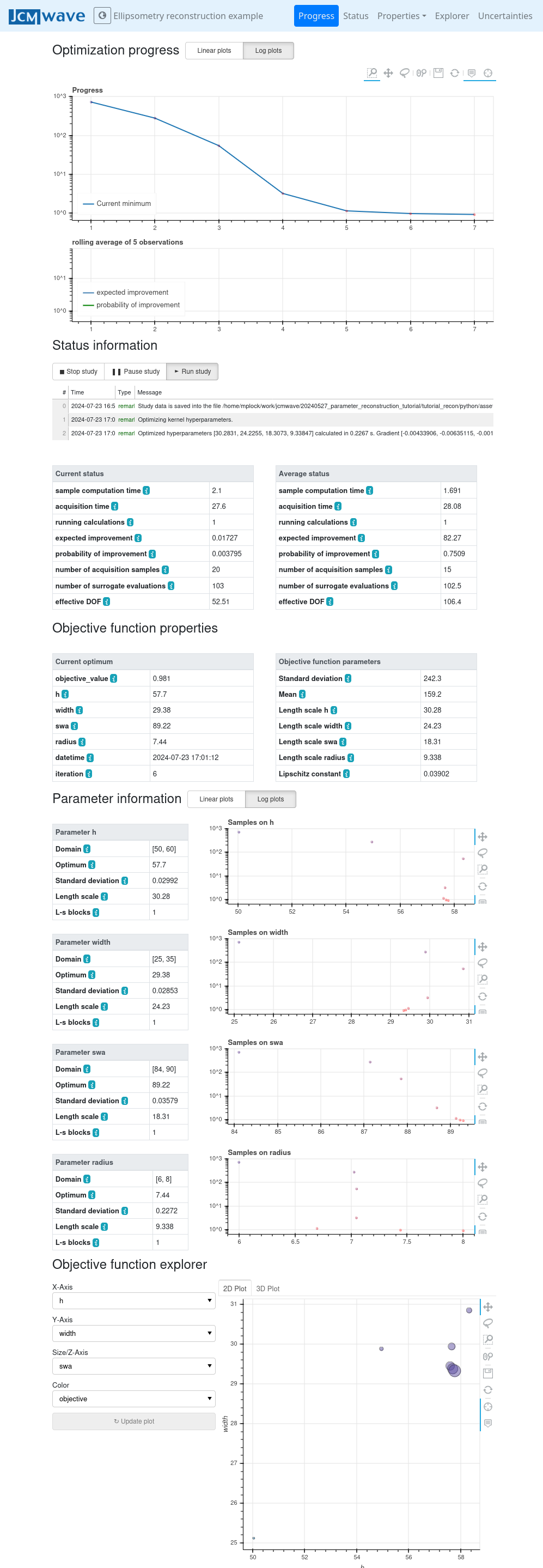
The parameter reconstruction reaches values close to 1 after only a few iterations.
After 20 iterations the Mueller matrix values have been sufficiently reconstructed.
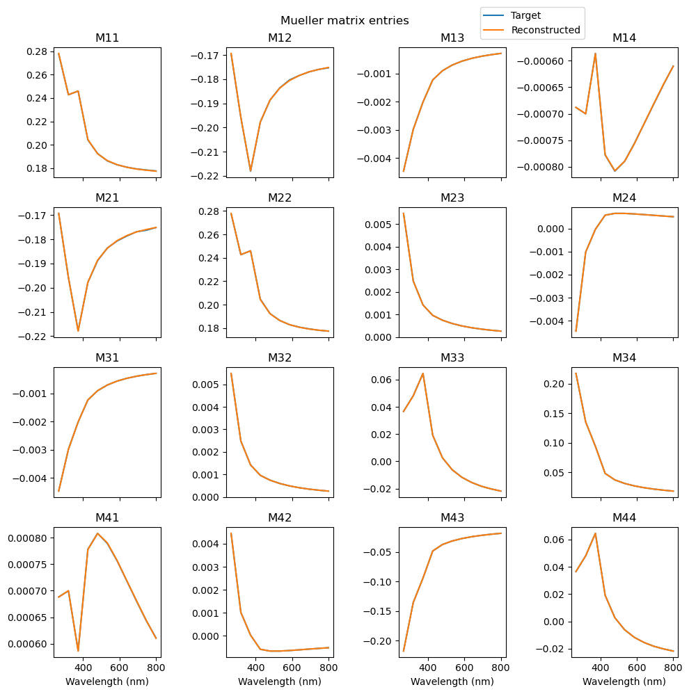
After 20 iterations the reconstructed Mueller matrix entries are indistinguishable from the target vector.