BesselBeam
| Type: | section |
|---|---|
| Appearance: | multiple |
Specifies a time-harmonic vectorial Bessel-Gaussian beam.
# define a Bessel beam with a propagating Fourier spectrum
BesselBeam {
  Incidence = FromBelow
  Lambda0 = 6.2831e-6
  SP = [1 0]
  ThetaPhi = [25 0]
  Focus = [0 0 0]
  Waist = 6.2831e-5
  Radial = 0.0174524064372835

  OpticalSystem {
    NumericalAperture = 1.0
  }
}
This section allows to specify the parameters of a vectorial Bessel-Gaussian beam defined by its Fourier spectrum. The following figure indicates the modeled setup of an incident beam passing through an optical system prior to reaching the computational domain.
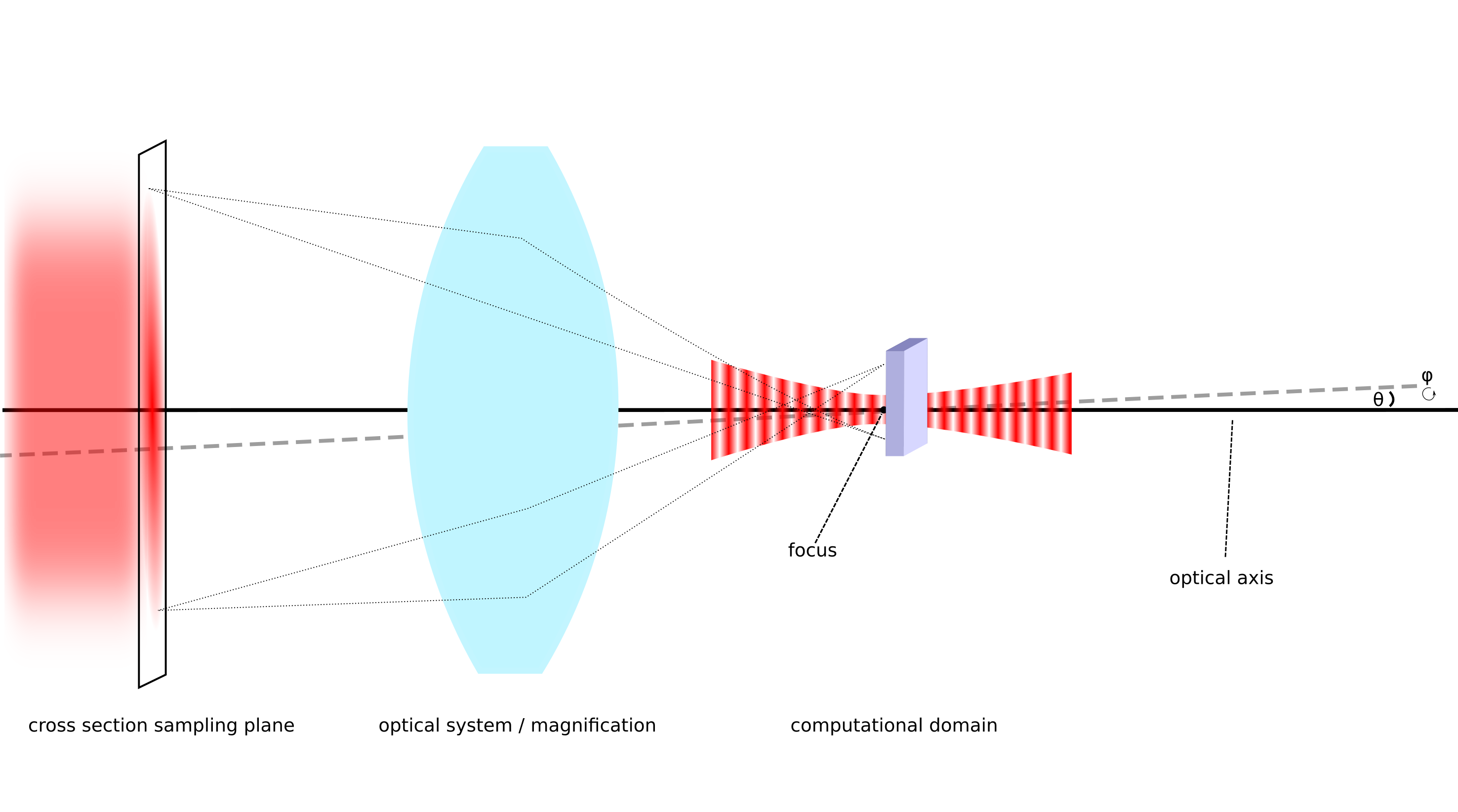
A macroscopic beam passes an optical system that focusses it into the computational domain. The beam is determined by its spatial distribution in the cross section plane in front of the optical system. The optical axis can tilted by the angles  and
and  .
.
The beam profile is determined by its spatial cross-section in a plane perpendicular to the optical axis and the optical system. The corresponding spectrum in k-space and the out of plane vector components are determined automatically.
Definition of the spatial cross section
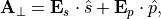
We use the 2-vector parameter SP, ![[\VField{\VField{E}}_s, \VField{\VField{E}}_p]](_images/math/b5f22d8018e807e1238a05ed391dd7e0db073ccf.png) to specify the polarization of the beam:
to specify the polarization of the beam:
where  are defined as for the plane wave case. This amplitude is modulated by a Bessel-Gaussian profile determined by the Waist, the Radial argument
  and the Order
  of the Bessel function of the first kind
  :
:
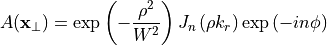
where the modulation depends on the radial coordinate 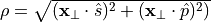 and azimuth .
The radial component is determined as the Radial fraction of the wavenumber
and azimuth .
The radial component is determined as the Radial fraction of the wavenumber 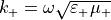 where
where  and
and  denote the corresponding scalar permittivity and permeability, respectively.
The resulting normalized intensity and phase distribution for various orders is shown in the figure below.

Left: Cross-section of the intensity distribution (normalized) for different orders. Right: Cross-section of the phase distribution.
Definition of the optical system
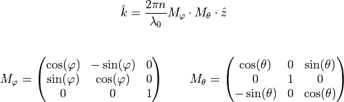
The OpticalSystem is used to model the transfer of the beam in the sampling cross section to the focal plane. The focal plane is described by the Focus and a rotation of the default optical axis  by the angles ThetaPhi. With the rotation matrices
  and
and  and the unit vector (the direction is determined by the parameter Incidence
  (
(FromBelow) or  (
(FromAbove) ) the optical axis  is calculated as follows:
.
The OpticalSystem has several parameters to describe aberrations as well as parameters defining the SpotMagnification and NumericalAperture to describe focusing system or restrict the Fourier spectrum.
Note
As the image is magnified by the value of SpotMagnification you must use a value  to describe a focusing system.
By default, the full Fourier spectrum is passed through a perfect system without abberations and an infinite numerical aperture.
Numerical parameters
The sampling rate is automatically adapted to suit the beam parameter. The parameter DeltaK and NRefinements can be used for a user-defined sampling.