Expression¶

Type:	string
Range:	[]
Default:	-/-
Appearance:	simple
Excludes:	Function, Module

This parameter is used to define a tensor field of type “relative permittivity” by means of a Python expression within the .jcm input file. The syntax is the following:

RelPermittivity {
  Python {
     Expression = " ... # your python scripting
                    ...
                    value = ... # set return value

                   "

     # define one or more parameters
     Parameter {
       Name = "Para1"
       ...
     }
     Parameter {
       Name = "Para2"
       ...

     }
  }
}

The string value Expression has to be valid Python code and is interpreted in the following way:

The NumPy-package is automatically imported when evaluating the expression.
Any parameter as defined by a Parameter section is available within the Python expression as an NumPy object named accordingly to the value of the parameter Name.
The position $\pvec{x}$ and the time $t$ are available as NumPy objects name X and t respectively.
For time-harmonic electromagnetic problems the angular frequency $\omega$ can be addressed by EMOmega, (EM stands for electromagnetic).
The expression must define a NumPy object named value which contains the return value of appropriate shape (relative permittivity is a $3 \times 3$ - matrix).
Keep in mind the Python indentation rule.

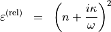
In a first practical example we want to give the $n, \kappa$ based definition of the relative permittivity, where $n$ denotes the refractive index and $\kappa$ the extinction factor. We want to assume that the relative permittivity is $\omega$ dependent in the following sense:

$\begin{eqnarray*} \TField{\varepsilon}^{(\mathrm{rel})} & = & \left( n+\frac{i\kappa}{\omega} \right)^2 \end{eqnarray*}$

The corresponding .jcm snippet may look like this:

RelPermittivity {
  Python {
    Expression = "value = pow(nk[0]+1j*nk[1]/EMOmega), 2)*eye(3, 3)"

    Parameter {
      Name = "nk"
      VectorValue = [..., ...] # set n,k here
    }
  }
}

As a second example we want to define a relative permittivity which varies with the temperature:

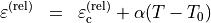
$\begin{eqnarray*} \TField{\varepsilon}^{(\mathrm{rel})} & = & \TField{\varepsilon}^{(\mathrm{rel})}_{\mathrm c} + \alpha (T-T_0) \end{eqnarray*}$

The first term is a constant value. The second term is a thermo-optical correction. This correction term has one field parameter - the temperature - and two coefficient parameters, the thermo-optical coefficient $\alpha$ and a standard temperature value $T_0$ .

The overall relative permittivity definition may be defined as:

RelPermittivity {
  Constant = ... # set first term eps_c, here
  Python {
    Expression = "value = a*eye(3, 3)*(T-T0)"

    Parameter {
      Name = "T"
      FieldValue {
        FieldBagPath = ... # path to a temperature field
        Quantity = Temperature
      }
    }
    Parameter {
      Name = "a"
      VectorValue = ... # scalar thermo-optical coefficient
    }
    Parameter {
      Name = "T0"
      VectorValue = ... # standard temperature
    }
  }
}