Scattering
| Type: | section |
|---|---|
| Appearance: | simple |
| Excludes: | PropagatingMode, ResonanceMode |
This section specifies scattering projects. Here, it is the aim to compute the electromagnetic field within a computational domain, excited by an illumination from outside or (/and) impressed currents.
An illuminating field is specified in the source file, sources.jcm, by its electric or magnetic field components. The following example declares an incoming plane wave:
SourceBag {

  # specify an illuminating
  Source {
   PlaneWave {
     K = [..., ..., ...]
     Amplitude = [..., ... , ...]
   }
}
The illuminating field is globally defined, i.e., the domain id, DomainId, is skipped. Physically, an illuminating plane wave corresponds to a far distance point source placed in the direction  of its wave vector and scaled to reach the origin with given amplitude. The wavenumber
  (also called angular wavenumber or circular wavenumber) refers to the material properties, i.e., permittivity and permeability, around the far distance source position as defined for the exterior domain.
To account for a complicated structured surrounding, such as a layered media, JCMsolve analyses the exterior domain and the illuminating field is computed accordingly. In case of a plane wave, the illuminating field comprises the multiple reflections and transmissions at the layer interface.
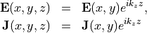
The angular frequency  is a fixed parameter and
 JCMsolve will determine it automatically by checking the impressed currents and the illumination. Similarly, in case of a periodic structure, the Bloch vector will be detected automatically.
Special geometries
2-dimensional, straight
When passing a two-dimensional grid file grid.jcm, JCMsolve treats the geometry as infinitely extended in the  -direction. It is required that the sources (impressed currents and illuminating fields) share the same harmonic dependence on the -coordinate:
JCMsolve detects the longitudinal phase factor  automatically from the prescribed sources.
3-dimensional, cylindrical
When the geometry exhibits a cylindrical symmetry with respect to the  -axis, it is possible to reduce the electromagnetic scattering computation to a series of separated two dimensional problems.
 JCMsolve will do this separation automatically, so that the cylindrical solver has no special settings compared to the full 3D setup.
Let  denote the cylindrical coordinates related to the Cartesian coordinates
  by
by

The material distribution is rotational symmetric when the permittivity tensor field  and the permeability tensor field
  satisfy
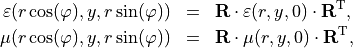
with the rotation matrix
![\begin{eqnarray*}
\TField{R} & = & \left [
\begin{array}{ccc}
\cos(\varphi) & 0 & -\sin(\varphi) \\
0 & 1 & 0 \\
\sin(\varphi) & 0 & \cos(\varphi) \\
\end{array}
\right ].
\end{eqnarray*}](_images/math/410217f6aece1b0c4f2f3692bba4b0bf66771372.png)
Hence, the device is fully described by the material distribution within the cross section  . Therefore,
 JCMsolve expects a two-dimensional grid file grid.jcm.
JCMsolve automatically expands the illuminating fields into Fourier series in  :
:
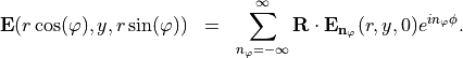
The impressed currents are treated accordingly. Then, Maxwell’s equations separate into a set of two-dimensional equations for each Fourier component. This yields a Fourier decomposition of the solution fields.
Based on error estimation, JCMsolve adaptively decides how many Fourier modes have to be taken into account in order to reach the demanded accuracy.