Illumination¶

Type:	section
Appearance:	optional

This section defines an extended, partially coherent illumination setup. Figure “illumination setup” is a simplified sketch of the situation as discussed in the parent section OpticalImaging.

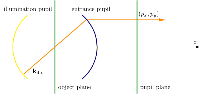
illumination setup¶

The system is illuminated by an extended light source (yellow sphere “illumination pupil”). For the moment, we assume that the space between the illumination and the entrance pupil is filled with a homogeneous medium. From each point of the illumination pupil a light ray of prescribed intensity is emitted (orange ray), which passes through the empty object plane (no scatterer, no mask blank), and which enters the optical system through the entrance pupil. This allows to identify the source point by its normalized pupil coordinates $(p_x, p_y)$ . 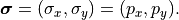In the context of the illumination system we switch to the notation $\boldsymbol\sigma = (\sigma_x, \sigma_y)=(p_x, p_y).$

We have assumed so far, that the space between the illumination system and the entrance pupil is homogeneous, so that the intensity of the ray on both sides of the object plane is unchanged. Hence, the light source specification may equally refer to the light source itself or to the image of the light source in the pupil plane, also called effective light source.

In reality the emitted light may pass a complicated condenser lens system before hitting the scatterer. Additionally, the system is often calibrated with a blank glass plate placed in the the object plane. Specifying the light source as an effective light source in the pupil plane abstracts the illumination source from its practical realization. This allows to cover reflective systems as well. We postpone this discussion to the section below. To discuss the coherence and polarization model first, we step back to the simple situation as sketched in Figure “illumination setup”.

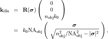
In the object plane, a source point $(\sigma_x, \sigma_y)$ corresponds to a plane wave which hits the scatterer under an incident angle of

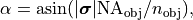
$\begin{eqnarray*} \alpha=\mathrm{asin}(|\boldsymbol \sigma| \mathrm{NA}_\mathrm{obj}/n_{\mathrm{obj}}), \end{eqnarray*}$

to the optical axis, and with the notation of the parent section OpticalImaging.

Defining the azimuthal angle 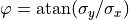$\varphi=\atan(\sigma_y / \sigma_x)$ , the corresponding $\pvec{k}-$ vector is given by

$\begin{eqnarray*} \pvec{k}_{\mathrm{illu}} & = & \TField{R}(\boldsymbol \sigma) \left ( \begin{array}{c} 0 \\ 0 \\ n_\mathrm{obj}k_0 \end{array} \right ) \\ { } & = & k_0 \mathrm{NA}_{\mathrm{obj}} \left ( \begin{array}{c} \boldsymbol \sigma \\ \sqrt{n_{\mathrm{obj}}^2/\mathrm{NA}_{\mathrm{obj}}^2-|\boldsymbol \sigma|^2} \end{array} \right ), \end{eqnarray*}$

with the rotation matrix 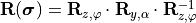$\TField{R}(\boldsymbol \sigma) = \TField{R}_{z, \varphi} \cdot \TField{R}_{y, \alpha} \cdot \TField{R}_{z, \varphi}^{-1}$ , where

$\begin{eqnarray*} \TField{R}_{z, \varphi} = \left ( \begin{array}{ccc} \cos(\varphi) & -\sin(\varphi) & 0 \\ \sin(\varphi) & \cos(\varphi) & 0 \\ 0 & 0 & 1 \end{array} \right ), \; \TField{R}_{y, \alpha} = \left ( \begin{array}{ccc} \cos(\alpha) & 0 & \sin(\alpha) \\ 0 & 1 & 0 \\ -\sin(\alpha) & 0 & \cos(\alpha) \end{array} \right ). \end{eqnarray*}$

Spatial coherence model

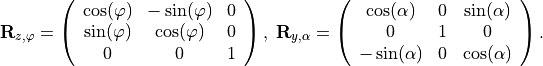
It is assumed that different source points are uncorrelated. Then, each illumination point $\boldsymbol \sigma$ gives independently rise to an intensity distribution in the image space,

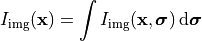
$\begin{eqnarray*} \boldsymbol \sigma \mapsto I_{\mathrm{img}}(\pvec{x}, \boldsymbol \sigma). \end{eqnarray*}$

Here, the computed intensity distribution may account for a stratification of the medium in the image space as set in Stratification. The total intensity is the integral over the entire source distribution:

$\begin{eqnarray*} I_{\mathrm{img}} (\pvec{x}) = \int I_{\mathrm{img}}(\pvec{x}, \boldsymbol \sigma)\,\dd \boldsymbol \sigma \end{eqnarray*}$

Polarization model

For a source point $\boldsymbol \sigma$ a polarized incoming plane wave can be specified by the complex-valued Jones vector 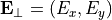$\pvec{E}_\perp = (E_x, E_y)$ int the pupil plane. The actual incoming field amplitude is then given by

$\begin{eqnarray*} \pvec{E}_{\mathrm{illu}, \perp} & = & \TField{R} \left ( \begin{array}{c} E_x \\ E_y \\ 0 \end{array} \right ). \end{eqnarray*}$

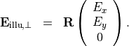
However, the incoming plane wave is often not fully polarized. Instead, the phases of $E_x$ and $E_y$ and their amplitudes may vary statistically. This necessitates to describe the polarization state of the incoming field by means of the polarization matrix (see [1], page 154)

$\begin{eqnarray*} \TField{P} = \left ( \begin{array}{cc} \langle E_x \Conj{E_x} \rangle & \langle E_x \Conj{E_y} \rangle \\ \langle E_y \Conj{E_x} \rangle & \langle E_y \Conj{E_y} \rangle \end{array} \right ), \end{eqnarray*}$

where $\langle \cdot \rangle$ denotes the time average. The entries the polarization matrix, $P_{kl}$ are the equal time cross-correlations of the field entries.

The intensity of the incoming plane wave is now given as the trace of the polarization matrix,

$\begin{eqnarray*} I_0 = \trace{\TField{P}}= \langle E_x \Conj{E_x} \rangle+\langle E_y \Conj{E_y} \rangle. \end{eqnarray*}$

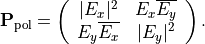
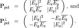
For completely polarized light the time-average becomes trivial and the polarization matrix is formed by the components of the Jones vector:

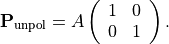
$\begin{eqnarray*} \TField{P}_{\mathrm{pol}} = \left ( \begin{array}{cc} |E_x|^2 & E_x \Conj{E_y} \\ E_y \Conj{E_x} & |E_y|^2 \end{array} \right ). \end{eqnarray*}$

For completely unpolarized light the correlation of $E_x$ and $E_y$ is zero. Since no preferred direction is allowed in the unpolarized case, the amplitudes $E_x$ and $E_y$ must equal. Hence, the polarization matrix is in diagonal from

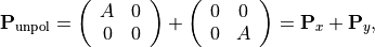
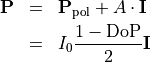
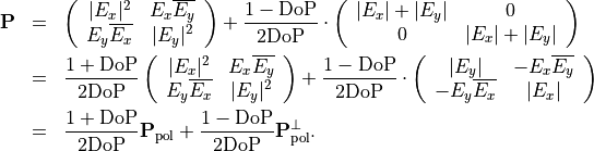
$\begin{eqnarray*} \TField{P}_{\mathrm{unpol}} = A \left ( \begin{array}{cc} 1 & 0 \\ 0 & 1 \end{array} \right ). \end{eqnarray*}$

In general, it can be shown that partially polarized light can be decomposed into an completely polarized state and a completely unpolarized state, (see [1], page 162),

$\begin{eqnarray*} \TField{P} = \TField{P}_{\mathrm{pol}}+\TField{P}_{\mathrm{unpol}} = \TField{P}_{\mathrm{pol}}+A \cdot \TField{Id}. \end{eqnarray*}$

This allows to define the degree of polarization as

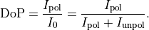
$\begin{eqnarray*} \mathrm{DoP} = \frac{I_\mathrm{pol}}{I_0} = \frac{I_\mathrm{pol}}{I_\mathrm{pol}+I_\mathrm{unpol}}. \end{eqnarray*}$

The coefficient $A$ is then determined from

$\begin{eqnarray*} 2 A = \trace{\TField{P}_\mathrm{unpol}} = \trace{\TField{P}}-\trace{\TField{P}_{\mathrm{pol}}}=(1-\mathrm{DoP}) \cdot I_0. \end{eqnarray*}$

Trivially, the unpolarized part can be split into two completely polarized states

$\begin{eqnarray*} \TField{P}_{\mathrm{unpol}} = \left ( \begin{array}{cc} A & 0 \\ 0 & 0 \end{array} \right ) + \left ( \begin{array}{cc} 0 & 0 \\ 0 & A \end{array} \right ) = \TField{P}_{x} + \TField{P}_{y}, \end{eqnarray*}$

so that the overall polarization state $\TField{P}$ is a sum of three contributions which independently passes the optical system in a coherent way.

Finally, the intensity distribution of a source point $\boldsymbol \sigma$ is the incoherent sum of three coherently formed intensities

In the appendix we derive an alternative decomposition of the polarization matrix $\TField{P}$ based on a decomposition into a incoherent sum of two completely polarized orthogonal states.

$\begin{eqnarray*} I_{\mathrm{img}}(\pvec{x}, \boldsymbol \sigma) = I_{\mathrm{img}, \mathrm{pol}}(\pvec{x}, \boldsymbol \sigma) + I_{\mathrm{img}, x}(\pvec{x}, \boldsymbol \sigma)+ I_{\mathrm{img}, y}(\pvec{x}, \boldsymbol \sigma). \end{eqnarray*}$

Effective light source

At the beginning of this section we have introduced the concept of an effective light source, which specifies the illumination as the image of the light source in the pupil plane formed by a reference system used for calibration with a blank glass plate in the object plane instead of a scatterer. This way, a complicated condenser lens system between the actual illumination and the object plane can be treated as a black box.

For a transmissive system, the situation is as depicted in Figure “transmissive mask blank”.

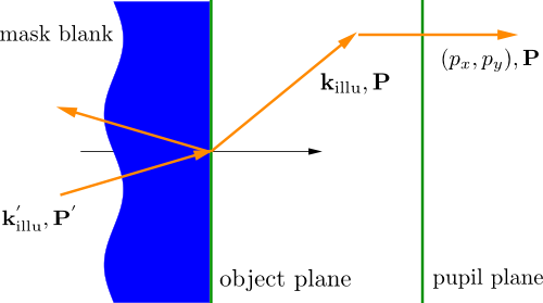
transmissive mask blank¶

The mask blank is colored in blue. It extends to infinity in $-z$ direction as indicated by the curved surface. In JCMsuite, the illumination specification refers to the rays within the pupil plane, e.g. they are specified by the normalized pupil coordinates $(p_x, p_y)$ and the polarization state $\TField{P}$ . Technically, one precisely specifies the measured image of the illumination in the pupil plane (effective source). The illuminating field ( $\pvec{k}_\mathrm{illu}^{'}$ , $\TField{P}^{'}$ ) as used in the near field computation is then backward-determined from Fresnel’s equations in case of a simple material interface mask blank $\leftrightarrow$ object space taking into account the object-sided obliquity factor $O_{\mathrm{obj}}(\pvec{p})$ and apodizations $e^{-2\pi d_{\mathrm{obj}}(\pvec{p})}$ . It is also possible to define a stratified mask blank, see BlankGeometry. T

A reflective system can be treated in a similar way, cf. Figure “reflective mask blank”.

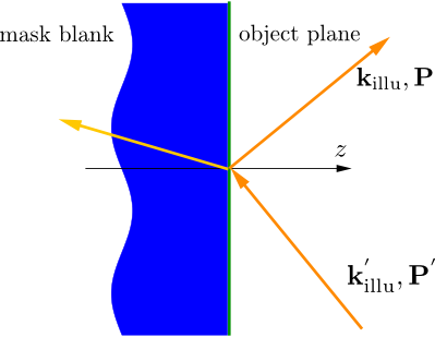
reflective mask blank¶

The object is illuminated from the side of the object plane, where the entrance pupil of the optical system is placed. Again, not the actual illuminating is specified ( $\pvec{k}_\mathrm{illu}^{'}$ , $\TField{P}^{'}$ ), but the effective source ( $(p_x, p_y)$ , $\TField{P}$ ) as it appears in the pupil plane after reflection off the blank.

Appendix

Decomposition into orthogonal states

For completely polarized light described by the Jones-vector $\TField{E}_{\mathrm{pol},\perp}=(E_x, E_y)$ one can define the orthogonal state as

$\begin{eqnarray*} \TField{E}^{\perp}_{\mathrm{pol},\perp}=(-\Conj{E_y}, \Conj{E_x}). \end{eqnarray*}$

Both states have equal intensities. The corresponding polarization matrices are given by

$\begin{eqnarray*} \TField{P}_{\mathrm{pol}} & = & \left ( \begin{array}{cc} |E_x|^2 & E_x \Conj{E_y} \\ E_y \Conj{E_x} & |E_y|^2 \end{array} \right ),\;\mbox{and} \\ \TField{P}^{\perp}_{\mathrm{pol}} & = & \left ( \begin{array}{cc} |E_y|^2 & -E_x \Conj{E_y} \\ -E_y \Conj{E_x} & |E_x|^2 \end{array} \right ). \end{eqnarray*}$

We want to transfer partially polarized light given as

$\begin{eqnarray*} \TField{P} & = & \TField{P}_{\mathrm{pol}}+A\cdot \TField{I} \\ {} & = & I_0 \frac{1-\mathrm{DoP}}{2} \TField{I} \end{eqnarray*}$

into an incoherent, weighted sum of the above orthogonal states. Using that

$\begin{eqnarray*} I_{\mathrm{pol}} = |E_x|^2+|E_y|^2=\mathrm{DoP}\cdot I_0, \end{eqnarray*}$

yields the desired decomposition:

$\begin{eqnarray*} \TField{P} & = & \left ( \begin{array}{cc} |E_x|^2 & E_x \Conj{E_y} \\ E_y \Conj{E_x} & |E_y|^2 \end{array} \right ) + \frac{1-\mathrm{DoP}}{2 \mathrm{DoP}} \cdot \left ( \begin{array}{cc} |E_x|+|E_y| & 0 \\ 0 & |E_x|+|E_y| \end{array} \right ) \\ {} & = & \frac{1+\mathrm{DoP}}{2 \mathrm{DoP}} \left ( \begin{array}{cc} |E_x|^2 & E_x \Conj{E_y} \\ E_y \Conj{E_x} & |E_y|^2 \end{array} \right ) + \frac{1-\mathrm{DoP}}{2 \mathrm{DoP}} \cdot \left ( \begin{array}{cc} |E_y| & - E_x \Conj{E_y} \\ -E_y \Conj{E_x} & |E_x| \end{array} \right ) \\ & = & \frac{1+\mathrm{DoP}}{2 \mathrm{DoP}} \TField{P}_{\mathrm{pol}}+ \frac{1-\mathrm{DoP}}{2 \mathrm{DoP}} \TField{P}^{\perp}_{\mathrm{pol}}. \end{eqnarray*}$

This equation can be brought into a more intuitive form when introducing the orthonormal states $\widehat{\TField{P}}_{\mathrm{pol}} = \TField{P}_{\mathrm{pol}}/I_\mathrm{pol}$ and $\widehat{\TField{P}}^{\perp}_{\mathrm{pol}} = \TField{P}^{\perp}_{\mathrm{pol}}/I_\mathrm{pol}$ :

$\begin{eqnarray*} \TField{P} & = & I_0 \cdot \left ( \frac{1+\mathrm{DoP}}{2} \cdot \widehat{\TField{P}}_{\mathrm{pol}}+ \frac{1-\mathrm{DoP}}{2} \cdot \widehat{\TField{P}}^{\perp}_{\mathrm{pol}} \right ). \end{eqnarray*}$

Bibliography

[1]	(1, 2) Wolf, E. Theory of Coherence and Polarization of Light, Cambridge 2007