PCESensitivityAnalysis
Purpose
The goal of the driver is to perform a variance based sensitivity analysis of a scalar function  or a vectorial function
  with respect to variations of a parameter vector
  . To this end, the function is decomposed into poylnomials using a polynomial chaos expansion (PCE).
Depending on the defined random distribution of each parameter (see parameter distribution), PCE uses different polynomials to obtain a good  convergence.
| Distribution of random variable | Polynomials
 |
|---|---|
| Uniform | Legendre |
| Gauss | Hermite |
| Gamma | Laguerre |
| Beta | Jacobi |
Using the default setting, the number of of expansion terms is chosen automatically based on a variance analysis of the model vector  .
.
The PCE can be used to predict the function and its derivatives with respect to each entry of the parameter vector  . Predictions can be computed by calling study.predict().
- There are two typical application scenarios of a variance based sensitivity analysis:
- The scalar function
 measures the performance of a device. The sensitivity analysis helps to quantify the average performance for random perturbations of the parameter vector . The analysis also quantifies which parameter combinations influence the performance .
 - The vectorial function
 describes a list of physical observables for parameter reconstruction. The analysis allows to identify vector entries with high sensitivity for specific parameters.
- The scalar function
The parameter vector consists of  entries, where each entry
  has a specific random distribution
  (see parameter distribution). Hence, the scalcar function is also a random variable (vectorial outputs are analysed by multiple independent sensitivity analyses).
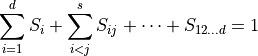
The variance of this random variable can analysed in terms of Sobol coefficients  . Each Sobol coefficient determines the fraction of the total variation that stems from the joint random variation of the parameters
  . The sum of all Sobol coefficients is 1,
For example, if  , then 10% of the variance of stem from the variance of an additive part
  of the function that only depends on the random variations of parameter
  and
and  . For more details on the definition of Sobol coefficients, see the section Additional Information.
Usage Example
addpath(fullfile(getenv('JCMROOT'), 'ThirdPartySupport', 'Matlab'));
client = jcmwave_optimizer_client();

% Definition of the search domain
domain = {
    struct('name','x1', 'type','continuous', 'domain',[-5,5]),...
    struct('name','x2', 'type','continuous', 'domain',[-5,5]),...
    struct('name','x3', 'type','continuous', 'domain',[-5,5]),...
};

% Creation of the study object with study_id 'example'
study = client.create_study('domain',domain,  ...
                'driver','PCESensitivityAnalysis',...
                'name','PCESensitivityAnalysis example', ...
                'study_id','PCESensitivityAnalysis_example');

% Definition of the objective function (Ishigami function)
a = 7; b = 0.1; %parameters of the Ishigami function
function obs = objective(sample)
  x1 = sample.x1;
  x2 = sample.x2;
  x3 = sample.x3;

  obs = study.new_observation();
  %objective
  obs = obs.add(sin(x1)+ a*sin(x2)^2 + b*x3^4*sin(x1));

end

% Define random distribution of parameters
distribution = {
    struct('name','x1', 'distribution','uniform', 'domain',[-pi,pi]),...
    struct('name','x2', 'distribution','uniform', 'domain',[-pi,pi]),...
    struct('name','x3', 'distribution','uniform', 'domain',[-pi,pi]) ...
};
% Set study parameters
study.set_parameters('max_iter',150, 'distribution',distribution);

% Run the study
while(not(study.is_done))
    sug = study.get_suggestion();
    obs = objective(sug.sample);
    study.add_observation(obs, sug.id);
end

%Analytic mean, variance and Sobol coefficients for the Ishigami function
mean = a/2;
variance = 1/2 + a^2/8 + b*pi^4/5 + b^2*pi^8/18;
sobol_values = struct(...
    'x1', 0.5*(1+b*pi^4/5)^2/variance,...
    'x2', (a^2/8)/variance,...
    'x1_x3', b^2*pi^8/2*(1/9-1/25)/variance...
);

driver_info = study.driver_info();
fprintf('\nMean %.3f Exact %.3f', driver_info.mean, mean);
fprintf('\nVariance %.3f Exact %.3f', driver_info.variance, variance);
fns = fieldnames(driver_info.sobol_indices);
for i=1:length(fns)
    sobol_index = driver_info.sobol_indices.(fns{i});
    val_driver = driver_info.sobol_coefficients.(fns{i});
    try
        val_exact = sobol_values.(fns{i});
    catch
        val_exact = 0;
    end
    fprintf('\nSobol index %s: %.3f Exact %.3f',mat2str(sobol_index),...
                                                val_driver,val_exact);
end
Parameters
The following parameters can be set by calling, e.g.
study.set_parameters('example_parameter1',[1,2,3], 'example_parameter2',true);
| max_iter (int): | Maximum number of evaluations of the objective function (default: inf) |
|---|
| max_time (int): | Maximum run time in seconds (default: inf) |
|---|
| num_parallel (int): | |
|---|---|
| Number of parallel observations of the objective function (default: 1) | |
| distribution (list): | |
|---|---|
Definition of random distribution for each parameter in the format of a list. All continuous parameters with unspecified distribution are assumed to be uniformely distributed in the parameter domain. Fixed and discrete parameters are not random parameters. The value of discrete parameters defaults to the first listed value. (default: None)
|
|
| sampling_strategy (string): | |
|---|---|
| Sampling strategy of parameter values. standard: Sampler for cartesian product samples of given parameters under algebraic constraints. WLS: Sampler for weighted Least-Squares sampling as described by Cohen and Migliorati. (default: WLS) (options: [‘standard’, ‘WLS’]) | |
| polynomial_degree (int): | |
|---|---|
| Maximum degree of the polynomial chaos expansion. Can be also a list of degrees for every parameter. If not set, the polynomial degree is iteratively adapted. (default: None) | |
| limit_polynomial_degree (int): | |
|---|---|
| Maximum sum of polynomial degree of the chaos expansion. (default: 2147483647) | |
| optimization_step (int): | |
|---|---|
| Number of iterations before the polynomial degrees of the expansion are optimized. Only applies if the polynomial degree is determined automatically (polynomial_degree=None). (default: 10) | |
| optimization_step_max (int): | |
|---|---|
| Maximum number of iterations after which the polynomial degrees of the expansion are optimized. Only applies if the polynomial degree is determined automatically (polynomial_degree=None). (default: 1000) | |
| pce_update_step (int): | |
|---|---|
| Number of iterations before the PCE is updated from the samples drawn so far. At each update, e.g. the values of the Sobol coefficients are updated. (default: 5) | |
| num_test_samples (int): | |
|---|---|
| Number of samples that are drawn in order to estimate the prediction error of the PCE. (default: 10) | |
| min_prediction_error (float): | |
|---|---|
| Stopping criterium. Minimum error of the prediction of the polynomial chaos expansion for the last 5 aqcuisitions. (default: 1e-06) | |
| target_cond (float): | |
|---|---|
| Target condition number of the information matrix. Only applies if the polynomial degree is determined automatically (polynomial_degree=None). (default: 500) | |
Driver-specific Information
A struct with following parameters can be retrieved by calling
study.driver_info().
| sobol_indices: | Dictionary mapping the names of Sobol indices (e.g. x1_x3) to the list of the corresponding parameter indices (e.g. [1,3]). |
|---|
| sobol_coefficients: | |
|---|---|
| Dictionary mapping the name of the Sobol indices (e.g. x1_x3) to the value of the Sobol coefficients. | |
| input_covariance: | |
|---|---|
Covariance matrix between entries of the vectorial input function , i.e. ![C_ij = \mathbb{E}\left[(f_i(\mathbf{p})-\overline{f}_i)(f_j(\mathbf{p})-\overline{f}_j)\right]](_images/math/c5a38ea82674a5ae8aed2d92ce0344ad813452c7.png) |
|
| predicition_error: | |
|---|---|
| Maximal predicion error of test data. | |
| num_expansion_terms: | |
|---|---|
| Number of PCE expansion terms. | |
| mean: | Mean of the objective functions under parameter uncertainties. |
|---|
| variance: | Variance of the objective functions under parameter uncertainties. |
|---|
Additional Information
Sobol coefficients
Each function can be decomposed into a unique sum called a Sobol decomposition,
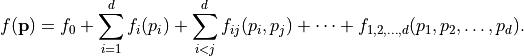
Here,  is a constant and each univariate integral over each term vanishes, i.e.

That is, all the terms in the functional decomposition are orthogonal.
The variance of the function is given as
![\text{Var}[f] = \int f^2(\mathbf{p}) \rho_1(p_1)\cdots\rho_d(p_d)\text{d}p_1\cdots\text{d}p_k - f_0^2.](_images/math/45bc7b0dc53f0f2fb7b543876b6a5c7692b7fe2e.png)
Due to the orthogonality, the variance can be decomposed into a sum of variances stemming from each term in the Sobol decomposition
![\text{Var}[f] = \sum_i \text{Var}[f_i] + \sum_{i<j} \text{Var}[f_ij] + \cdots + \text{Var}[f_{1 2\dots d}]](_images/math/e064b99e65451a73493c4f57ffcf95b5fc7382b5.png)
where
![\text{Var}[f_{i_1,i_2,\dots,i_s}] = \int f_{i_1,i_2,\dots,i_s}^2(p_{i_1},p_{i_2},\dots,p_{i_s}) \rho_{i_1}(p_{i_1})\cdots\rho_{i_s}(p_{i_s})\text{d}p_{i_1}\cdots\text{d}p_{i_s}.](_images/math/fd7f161d8dc68b395ae0638702e0f051b61b4ce9.png)
The Sobol coefficient is defined as the fraction of the total variance that stems from the additive term  , i.e.
![S_{i_1,\dots,i_s} = \frac{\text{Var}[f_{i_1,i_2,\dots,i_s}]}{\text{Var}[f]}.](_images/math/1479a5ff0d9f368fb80a33ba2210737e77e12188.png)