Optimization
In order to use the new JCMoptimizer MATLAB interface, please follow the instructions in the JCMoptimizer Matlab documentation to install the interface for the new optimizer. The new interface (+jcmoptimizer) is placed in this directory.
In this section we present a way to efficiently optimize an optical structure. The optimization algorithm is based on a Bayesian optimization approach [Schn2017], which requires substantially fewer simulation results than other optimization algorithms [Schn2019]. As an example we revisit the structure with a square unit cell discussed in the EM-tutorial. The goal of the optimization is to create a silicon metasurface with a minimal reflectivity, which can act as an antireflective coating. The design and fabrication of such a coating has been discussed in [Prou2016].
We consider a periodic grating with square-like structures. The variable parameters of the system are shown in the figure below.
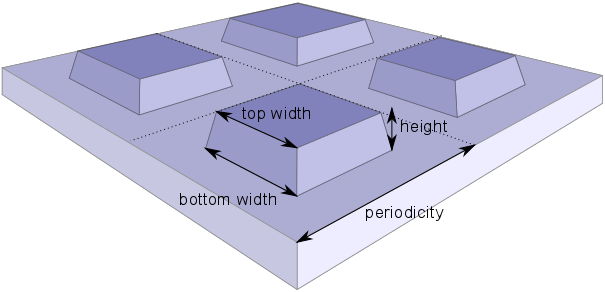
The metasurface is parametrized by the periodicity, the height of the etched structures, their bottom, and their top widths.
First, we define the search domain for the minimization of the reflectivity:
domain = {};
domain(1).name = 'height';
domain(1).domain = [50,200];
domain(2).name = 'bottom_width';
domain(2).domain = [60,200];
domain(3).name = 'top_width';
domain(3).domain = [60,200];
domain(4).name = 'periodicity';
domain(4).domain = [150,400];
The bottom and top widths may not exceed the periodicity of the structure. Hence, we have to define two constraints of the search domain. A constraint is defined by a function expression that returns a negative value, if and only if the constraint is fulfilled.
constraints = {};
constraints(1).name = 'max_bottom_width';
constraints(1).expression = 'bottom_width - periodicity + 10';
constraints(2).name = 'max_top_width';
constraints(2).expression = 'top_width - periodicity + 10';
With the domain and constraints variables one can now create a new study object. We set the maximal number of optimization iterations to 20. The Matlab interface currently runs one optimizer evaluation at a time, so num_parallel is set to 1.
% Creation of the study object
server = jcmoptimizer.Server("server_location", "local");
client = jcmoptimizer.Client('host', server.host);

study = client.create_study( ...
    'design_space', domain, ...
    'constraints', constraints,...
    'driver','BayesianOptimization',...
    'study_name','Bayesian optimization',...
    'study_id', 'bayesian_optimization', ...
    'save_dir', '.');

% The MATLAB interface does not support parallel execution
study.configure('max_iter', 20, 'num_parallel', 1);
Before the objective function is evaluated, we start up the daemon. Details on how to use the daemon are described in the tutorial Parallel Parameter Scan.
% Startup daemon
jcmwave_daemon_startup();
jcmwave_daemon_add_workstation('Hostname', 'localhost', ...
				       'Multiplicity', 1, ...
				       'NThreads', 1);
Next, we define the objective function, that computes the reflectivity of the metasurface based on the Fourier coefficients in Z direction [*]. The convergence of the optimization can be largely improved by providing also derivative information. To this end the derivatives of the Fourier coefficients are calculated by the solver as described in this tutorial example . The objective function returns an observation object containing the objective value and its derivatives.
function observation = objective(study, sample, lambdas, permittivities, domain)

    job_ids = [];
    keys = sample;
    keys.slc = 150;
    for ii = 1 : numel(lambdas)
        keys.lambda0 = lambdas(ii)*1e-9;
        keys.permittivity = permittivities(ii);
        job_id = jcmwave_solve('project.jcmp', keys, 'temporary', 'yes');
        job_ids(end+1) = job_id;
    end

    [results, logs] = jcmwave_daemon_wait(job_ids);

    refl = 0;
    derivatives = zeros(numel(domain),1);
    pref = 1/numel(lambdas);
    for ii = 1 : numel(lambdas)
        FC = results{ii}{2}.ElectricFieldStrength{1};
        this_refl = sum(real(FC).^2 + imag(FC).^2);
        refl = refl + pref*this_refl;
        for jj = 1 : numel(domain)
            dfT = getfield(results{ii}{2},['d_' domain(jj).name]);
            dFC = dfT.ElectricFieldStrength{1};
            d_this_refl = sum(2*(real(FC).*real(dFC) + imag(FC).*imag(dFC)));
            derivatives(jj) = derivatives(jj) + pref*d_this_refl;
        end
    end

    observation = study.new_observation();
    observation.add(refl);
    for ii = 1 : numel(domain)
        observation = observation.add(derivatives(ii), 'derivative', domain(ii).name);
    end

end
Finally, we register the objective function as the evaluator of the study and
start the optimization. The study then handles the acquisition loop: it proposes
new parameter values, evaluates the objective function, and stores the returned
observations. The Matlab callback passes the wavelength list, material
permittivities, and search domain to the objective function explicitly. The number
of simultaneous optimizer evaluations is controlled by the num_parallel
setting configured above.
% The reflectivity is averaged over the wavelengths 600nm 700nm 800nm
lambdas = [600 700 800];
permittivities = [15.590 + 0.21635j 14.317 + 0.092101j 13.646 + 0.048345j];


% Run the minimization; extend the function signature of the objective
% function to include the additional parameters
study.set_evaluator(@(study, sample) objective( ...
    study, sample, lambdas, permittivities, domain));
study.run();
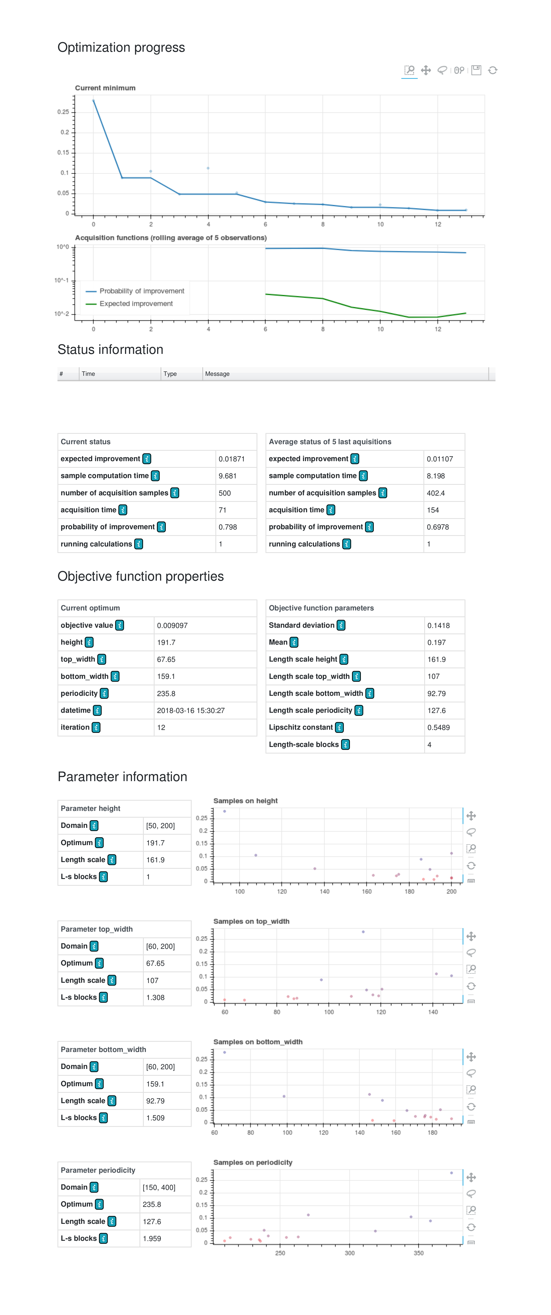
The progress of the optimization can be examined in a dashboard, that is shown in a browser window. A typical example is shown in the figure below. By optimizing the parameters one can reduce the reflectivity from 30% to below 1%.
Input Files
| [*] | To speed up the computation times for this tutorial example, we set the side length constraint of the mesh to 150nm (keys['slc']=150). In order to obtain converged results, one should rather use a value of 40nm. |
| [Schn2019] | P.-I. Schneider, X. Garcia Santiago, V. Soltwisch, M. Hammerschmidt, S. Burger, C. Rockstuhl. Benchmarking Five Global Optimization Approaches for Nano-optical Shape Optimization and Parameter Reconstruction ACS Photonics 6, 2726 (2019) https://doi.org/10.1021/acsphotonics.9b00706 https://arxiv.org/abs/1809.06674 |
| [Schn2017] | P.-I. Schneider, X. Garcia Santiago, C. Rockstuhl, S. Burger. Global optimization of complex optical structures using Bayesian optimization based on Gaussian processes Proc. SPIE 10335 (2017) 103350O (2017) https://doi.org/10.1117/12.2270609 https://arxiv.org/abs/1707.08479 |
| [Prou2016] | Julien Proust, Anne-Laure Fehrembach, Frédéric Bedu, Igor Ozerov and Nicolas Bonod. Optimized 2D array of thin silicon pillars for efficient antireflective coatings in the visible spectrum. Scientific Reports volume 6, Article number: 24947 (2016) http://dx.doi.org/10.1038/srep24947 |