Parameter Scan

With the parameterization of the test project in the previous section Keyword Substitution, it is straightforward to run a parameter scan within Matlab:

%% holds computed scattering cross sections
scattering_cross_section_scan = [];

%% loop over radius values
for radius = [0.3 : 0.005 : 0.5]  
  fprintf('\nSolving for radius %5.2e', radius);

  % set current parameter and solve the project
  keys.radius = radius;
  results = jcmwave_solve('mie2D.jcmp', keys, 'logfile', 'null');

  scs = real(results{2}.ElectromagneticFieldEnergyFlux{1});

  % gather results
  scattering_cross_section_scan(end+1, 1 : 2) = [radius, scs];
end

%% plot scattering cross section against rod radius
radii = scattering_cross_section_scan(:, 1);
scs = scattering_cross_section_scan(:, 2);
plot(radii, scs, '-+', 'LineWidth', 2);
xlabel('radius [\mu m]', 'FontSize', 14);
ylabel('integral scattering cross section', 'FontSize', 14);
set(gca, 'FontSize', 14);

In line 2 we initialize the matrix scattering_cross_section_scan which later holds the computed data. In line 5 we start a loop over the rod radius. In each step the key-value container keys is updated with the current radius value (line 9), followed by a solver call (line 10). The optional parameter logfile redirects the solver console output to a file (using null disregards all console output). In line 15 we gather the relevant data. Line 19-24 serve the plotting of the results, see Figure “Scattering Cross Section”.

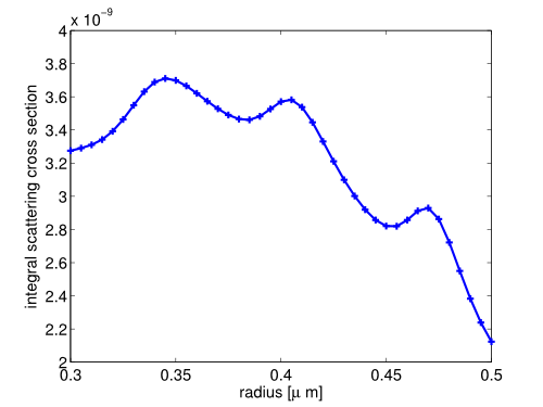
Scattering Cross Section

Computed scattering cross section versus rod radius.

The next section Matlab Code Snippets demonstrates how to enrich the .jcmt input files with matlab scripts blocks.