Transparent and mirror boundaries
Learning targets
- Specify different conditions at different boundaries of the computational domain
This geometry example specifies a rectangular computational domain
with Mirror boundary identifiers at the left and right side of the
computational domain and transparent boundaries at the upper and lower
side of the computational domain. This is a typical situation for
light scattering simulations with periodic scattering objects (e.g.,
diffraction grating) where the size of the computational domain
can be reduced by a factor of 2 when symmetry considerations about
the geometry and the source are taken into account.
The resulting geometry and mesh correspond to the following figure:
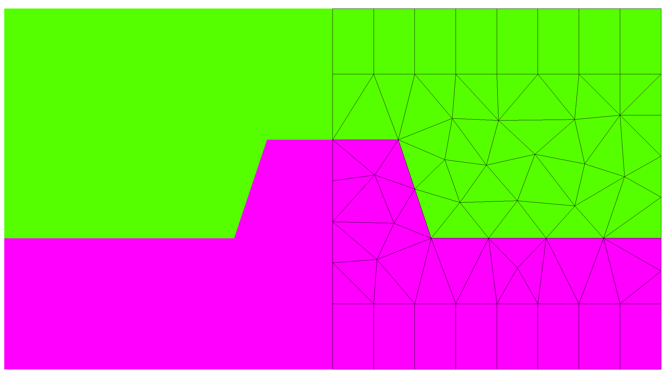
The geometry is automatically unfolded by JCMview. Only shown mesh elements are present in the grid.
.jcm Input File
layout.jcm [ASCII]
 1
 2
 3
 4
 5
 6
 7
 8
 9
10
11
12
13
14
15
16
17
18
19
20
21
22
23
24
25
26
27
28
29
30
31
32
Layout2D {
  Name = "GeometryTutorial2D/Grating"
  UnitOfLength = 1e-06

  MeshOptions {
    MinimumMeshAngle = 20
    MaximumSideLength = 1.2
  }
  Objects {
    Polygon {
      Name = "ComputationalDomain/Background"
      DomainId = 1
      Priority = -1
      Points = [0 -1, 5 -1, 5 2.5, 0 2.5]
      Boundary {
        Number = [1 3]
        Class = Transparent
      }
      Boundary {
        Number = [2 4]
        Class = Mirror
      }
    }

    Polygon {
      Name = "DielectricMaterial"
      DomainId = 2
      Priority = 1
      Points = [5 -1, 5 0, 1.5 0, 1 1.5, -1 1.5, -1.5 0, -5 0, -5 -1]
    }
  }
}
Here, the two mirror planes effectively model a periodic grating. To obtain an isolated grating line with symmetry all we need to do is a slight adaptation of the boundary condition settings:
Polygon {
    ...

    Boundary {
      Number = [1 2 3]
      Class = Transparent
    }
    Boundary {
      Number = 4
      Class = Mirror
    }
  }