Nanosphere
This tutorial example simulates light scattering off a spherical particle above a substrate.
The particle is illuminated with plane waves at oblique incidence, with S- and P-polarization.
JCMsuite computes the near-field solution.
Post-processes are used to compute absorption and scattering cross-sections, and to export field profiles.
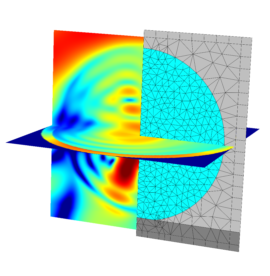
Near field intensity (pseudo-color, log-scale) in two cross-sections and triangular mesh of the geometry.
Definition of the geometry:
layout.jcm [ASCII]
 1Layout2D {
 2  UnitOfLength = 1e-09
 3  MeshOptions {
 4    MaximumSideLength = 100
 5  }
 6  CoordinateSystem = Cylindrical
 7  BoundaryConditions {
 8    Boundary {
 9      Direction = All
10      Class = Transparent
11    }
12  }
13  Objects {
14    Parallelogram {
15      Name = "CD"
16      Height = 900
17      Width = 450
18      Port = West
19      GlobalPosition = [0 0]
20      DomainId = 1
21      Priority = ComputationalDomain
22    }
23    CircleSector {
24      Radius = 400
25      AngleRange = [-90 90]
26      GlobalPosition = [0 0]
27      DomainId = 2
28      Priority = 1
29      RefineAll = 4
30      MeshOptions {
31        MaximumSideLength = 50
32      }
33    }
34
35    Parallelogram {
36      Height = 900
37      Width = 450
38      Port = North
39      Alignment {
40        Parent {
41          Domain = "CD"
42          Port = South
43        }
44        Displacement = [-0 -60]
45        Orientation = AntiParallel
46      }
47      DomainId = 3
48      Priority = 2
49
50    }
51  }
52}
The computational domain is defined by a parallelogram in the x-y-plane. In line 6 the coordinate system is chosen which defines the y-axis as rotational symmetry axis. The sphere is defined by a (rotated) circle sector (lines 23-33), and the substrate is defined by a (rotated) parallelogram.
The refractive indices, resp. relative permittivities, of the various geometrical domains are defined here:
materials.jcm [ASCII]
 1Material {
 2  DomainId = 1
 3  RelPermittivity = 1
 4  RelPermeability = 1
 5}
 6Material {
 7  DomainId = 2
 8  RelPermittivity = (8.99, 0.6)
 9  RelPermeability = 1
10}
11Material {
12  DomainId = 3
13  RelPermittivity = 2.25
14  RelPermeability = 1
15}
16
The illumination with two independent, S- and P-polarized plane waves is defined in the following:
sources.jcm [ASCII]
 1
 2SourceBag {
 3  Source {
 4    ElectricFieldStrength {
 5      PlaneWave {
 6        Lambda0 = 4e-07
 7        ThetaPhi = [20 0]
 8        Incidence = FromAbove
 9        3DTo2D = yes
10        SP = [1 0]
11
12      }
13    }
14  }
15}
16SourceBag {
17  Source {
18    ElectricFieldStrength {
19      PlaneWave {
20        Lambda0 = 4e-07
21        ThetaPhi = [20 0]
22        Incidence = FromAbove
23        3DTo2D = yes
24        SP = [0 1]
25      }
26    }
27  }
28}
29
Project type, accuracy settings and several post-processes are defined in the project file:
project.jcmp [ASCII]
 1Project {
 2  Electromagnetics {
 3    TimeHarmonic {
 4      Scattering {
 5        FieldComponents = Electric
 6        Accuracy {
 7          FiniteElementDegree = 3
 8        }
 9      }
10    }
11  }
12}
13PostProcess {
14  DensityIntegration {
15    FieldBagPath = "project_results/fieldbag.jcm"
16    OutputFileName = "project_results/energy.jcm"
17    OutputQuantity = ElectricFieldEnergy
18  }
19}
20PostProcess {
21  FluxIntegration {
22    FieldBagPath = "project_results/fieldbag.jcm"
23    OutputFileName = "project_results/scattered_energy_flux.jcm"
24    OutputQuantity = ElectromagneticFieldEnergyFlux
25    InterfaceType = ExteriorDomain
26  }
27}
28PostProcess {
29  ExportFields {
30    FieldBagPath = "project_results/fieldbag.jcm"
31    OutputFileName = "project_results/c_xy.jcm"
32    Cartesian {
33      GridPointsX = [-447.5e-9 : 5e-9 : 450e-9]
34      GridPointsY = [-450.0e-9 : 5e-9 : 450e-9]
35      GridPointsZ = 0
36    }
37  }
38}
39PostProcess {
40  ExportFields {
41    FieldBagPath = "project_results/fieldbag.jcm"
42    OutputFileName = "project_results/c_xz.jcm"
43    Cartesian {
44      GridPointsX = [-447.5e-9 : 5e-9 : 450e-9]
45      GridPointsZ = [-450.0e-9 : 5e-9 : 450e-9]
46      GridPointsY = 0
47    }
48  }
49}
The density integration post-process can be used to compute the absorption cross-section.
The flux integration post-process can be used to compute the scattering cross-section.
(Alternatively, also far-field computation / Fourier transform post-process can be used for
obtaining angular dependent scattering amplitudes.)
ExportFields post-processes are used for visualization purposes in this case.
The data_analysis folder contains also a script where geometrical, material, source, and computational parameters can be set, and where a wavelength scan is performed, yielding computation of the wavelength dependent absorption and scattering cross-sections (with corresponding template files layout.jcmt, sources.jcmt, materials.jcmt, project.jcmpt).
Please note that in this case JCMsuite is used in Daemon mode, allowing for parallel execution of the various wavelengths of the wavelength scan.
With appropriate hardware and license, all wavelength responses can be computed at the same time, allowing for fast computation of the whole parameter scan.
data_analysis/run_simulation.m [ASCII]
 1local_jcm_path = getenv('JCMROOT'); addpath(fullfile(local_jcm_path, 'ThirdPartySupport', 'Matlab'));
 2jcmwave_startup; jcmwave_set_num_threads(1); jcmwave_daemon_shutdown();
 3jcmwave_daemon_add_workstation('Multiplicity', 2, 'NThreads', 1);
 4
 5% geometry
 6keys.uol = 1.e-9;
 7keys.radius_scatterer = 400.0;
 8keys.contains_substrate = true;
 9keys.offset_sphere = -10.0; % offset between sphere and substrate in uol
10
11% refractive indices
12keys.n_1 = 1.0; % background
13keys.n_2 = 3.0 + 0.1i; % sphere
14keys.n_3 = 1.5; % substrate
15
16% S&P plane waves incidence angle
17keys.theta = 20;
18
19keys.fem_degree = 3;
20keys.n_steps = 0;
21
22c0 = 299792458; mu0 = 4*pi*1e-7; eps0 = 1/(mu0*c0^2); Z0 = sqrt(mu0/eps0);
23geo_cross_section = pi*(keys.radius_scatterer*keys.uol)^2; p_in = 0.5*keys.n_1/Z0*geo_cross_section;
24
25% parameter scan
26job_ids = []; results = []; simulation_results = []; counter = 0;
27
28wavelengths = [400:2:600]*1e-9;
29
30for ii = 1:length(wavelengths)
31  counter = counter + 1;
32  keys.vacuum_wavelength = wavelengths(ii);
33
34  job_ids(end + 1) = jcmwave_solve('project.jcmp', keys, 'workingdir', fullfile('tmp', ['s_' num2str(counter, '%05i')]));
35
36  results(counter, 1) = keys.vacuum_wavelength;
37  results(counter, 6) = keys.fem_degree;
38  results(counter, 7) = keys.n_steps;
39end;
40
41[simulation_results, logs] = jcmwave_daemon_wait(job_ids);
42
43for ii = 1:length(job_ids)
44  this_result = simulation_results{ii};
45  field_energy = cell2mat(this_result{2}.ElectricFieldEnergy);
46  omega = 2*pi*c0/keys.vacuum_wavelength;
47  absorption = -2*omega*imag(field_energy(2, :))/p_in;
48  flux_scat = cell2mat(this_result{4}.ElectromagneticFieldEnergyFlux);
49  scattering = sum(real(flux_scat), 1)/p_in;
50  results(ii, 2:3) = absorption;
51  results(ii, 4:5) = scattering;
52end
53
54filename = ['results_' datestr(now,'yyyymmdd_HHMMSS') '.txt'];
55save ('-ascii', '-double', filename, 'results'); copyfile(filename, 'results.txt');
56display_results;
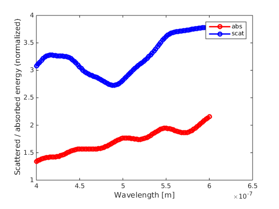
Wavelength-dependent absorption and scattering off a nanosphere on top of a substrate.