Isolated Slit and Groove
This tutorial example follows a benchmark setup investigated by P. Lalanne et al. [1]. Performance of FEM for the same setup has also been demonstrated [2]. The benchmark setup consists of computing the near field in an isolated (i.e., non-periodic) pattern illuminated by a plane wave. The geometry consists of an isolated, sub-wavelength slit in a silver film on a substrate with a neighboring, parallel groove in the silver film. This setup is illuminated by a plane wave at perpendicular incidence from above and with in-plane electric field polarization (resp. out-of-plane magnetic field polarization). The energy flux of light transmitted through the slit to a detector region placed a specific distance below the slit is detected and normalized to the energy flux through the slit, computed in a second simulation where the groove is not present. Due to the geometrical, source and material properties plasmonic effects lead to a very critical dependence of normalized transmission on the physical parameters. This makes accurate computation of normalized transmission a challenging benchmark problem.
|
|
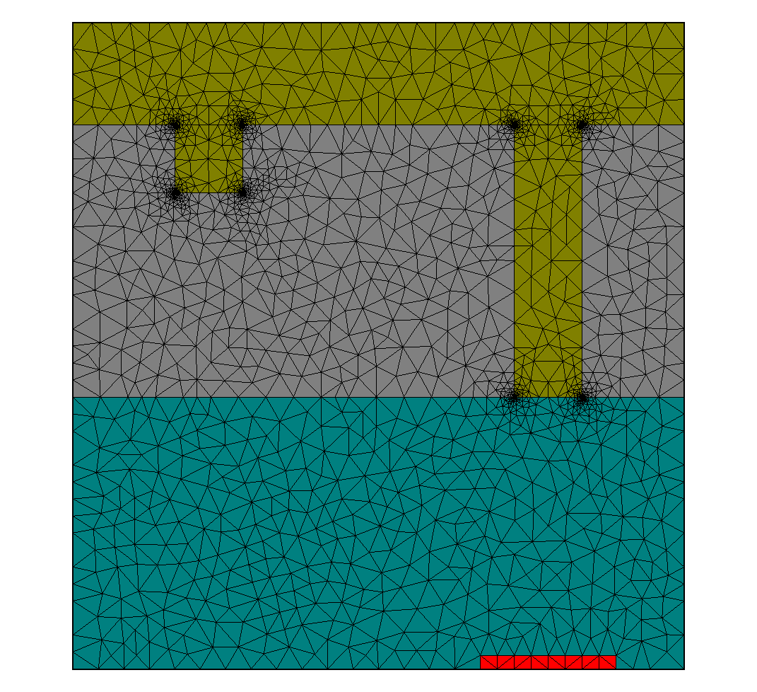
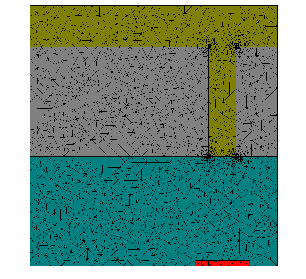
|
|
|
|
 , bottom row:
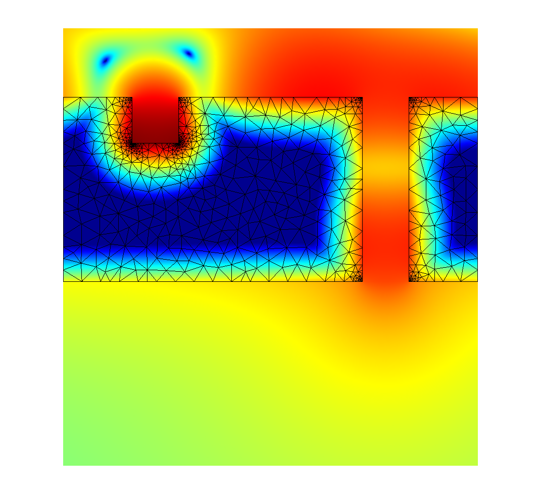
  , pseudo color scale):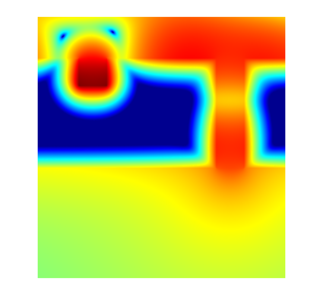
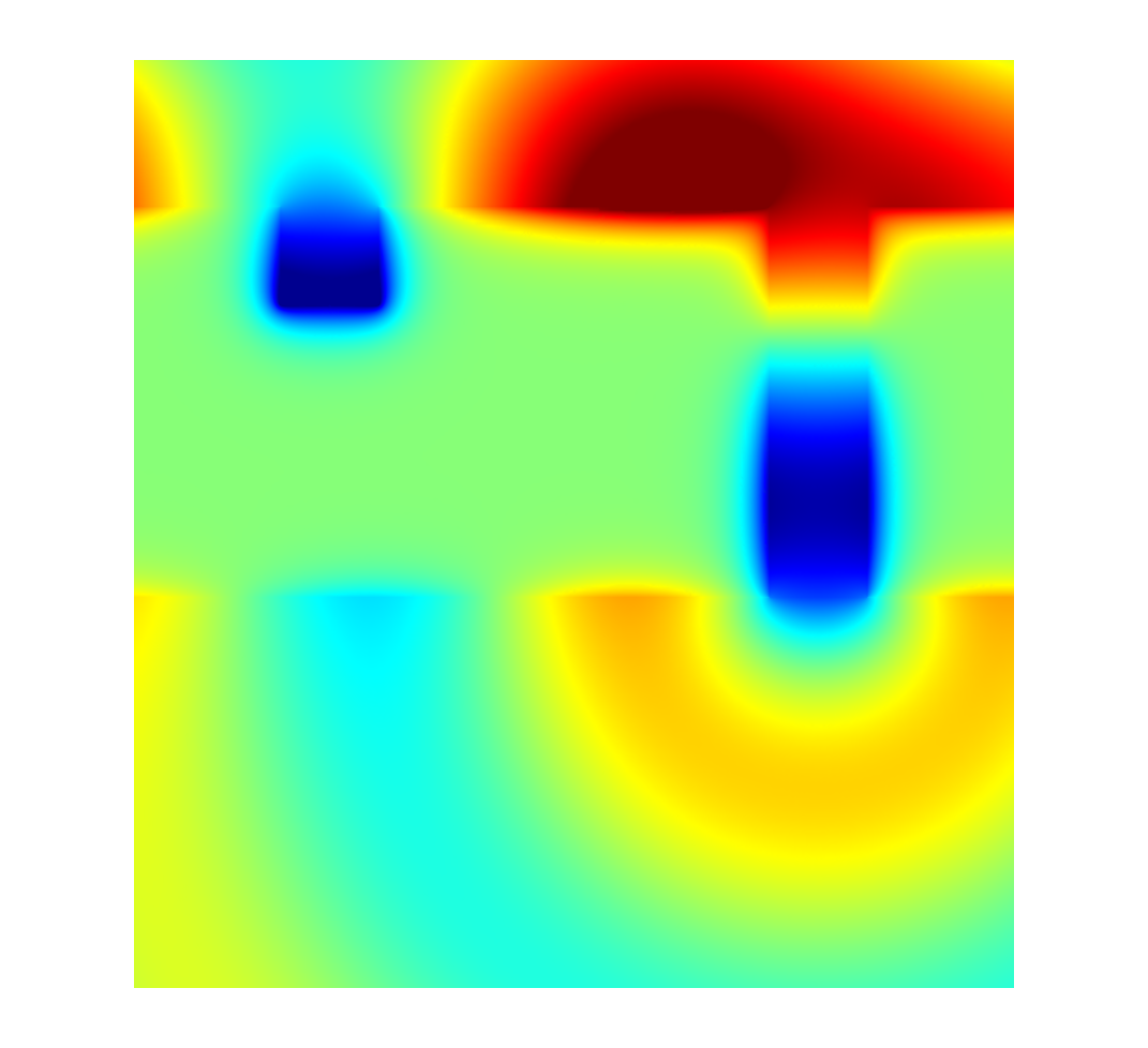
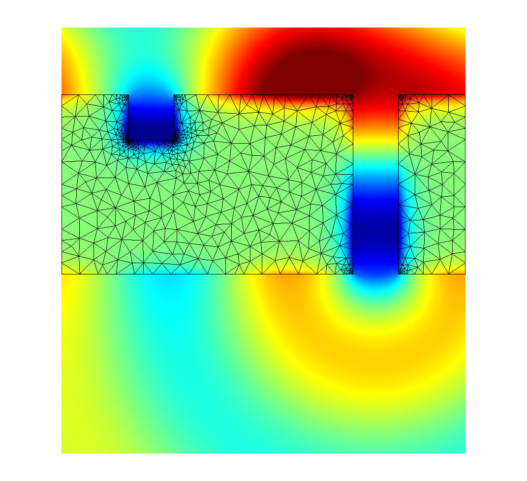
Definition of the geometry (please note CornerRefinement in the definitions for slit and groove):
layout.jcm [ASCII]
  1Layout2D {
  2  UnitOfLength = 1e-09
  3  MeshOptions {
  4    MinimumMeshAngle = 28
  5    MaximumSideLength = 50
  6  }
  7  Objects {
  8    Parallelogram {
  9      Name = "CD"
 10      DomainId = 1
 11      Priority = ComputationalDomain
 12      Width = 900
 13      Height = 950
 14      Boundary {
 15        Class = Transparent
 16      }
 17    }
 18    Parallelogram {
 19      Name = "Substrate"
 20      DomainId = 2
 21      Priority = 3
 22      Width = 900
 23      Height = 400
 24      Port = South
 25      Alignment {
 26        Parent {
 27          Domain = "CD"
 28          Port = South
 29        }
 30        Orientation = Parallel
 31        Displacement = [0 0]
 32      }
 33    }
 34    Parallelogram {
 35      Name = "Ag"
 36      DomainId = 3
 37      Priority = 2
 38      Width = 900
 39      Height = 400
 40      Port = South
 41      Alignment {
 42        Parent {
 43          Domain = "Substrate"
 44          Port = North
 45        }
 46        Orientation = AntiParallel
 47        Displacement = [0 0]
 48      }
 49    }
 50    Parallelogram {
 51      Name = "Groove"
 52      DomainId = 1
 53      Priority = 4
 54      Width = 100
 55      Height = 100
 56      Port = North
 57      Alignment {
 58        Parent {
 59          Domain = "Ag"
 60          Port = North
 61        }
 62        Orientation = Parallel
 63        Displacement = [250 0]
 64      }
 65      MeshOptions {
 66        CornerRefinement {
 67          MaximumSideLength = 0.1
 68          Progression = 3
 69        }
 70      }
 71    }
 72    Parallelogram {
 73      Name = "Slit"
 74      DomainId = 1
 75      Priority = 4
 76      Width = 100
 77      Height = 400
 78      Port = North
 79      Alignment {
 80        Parent {
 81          Domain = "Ag"
 82          Port = North
 83        }
 84        Orientation = Parallel
 85        Displacement = [-250 0]
 86      }
 87      MeshOptions {
 88        CornerRefinement {
 89          MaximumSideLength = 0.1
 90          Progression = 3
 91        }
 92      }
 93    }
 94    Parallelogram {
 95      Name = "Detector"
 96      DomainId = 4
 97      Priority = 4
 98      Width = 200
 99      Height = 20
100      Port = South
101      Alignment {
102        Parent {
103          Domain = "Slit"
104          Port = South
105        }
106        Orientation = Parallel
107        Displacement = [0 -400]
108      }
109    }
110  }
111}
Definition of material properties:
materials.jcm [ASCII]
 1
 2Material {
 3  Name = "Air"
 4  DomainId = 1
 5  RelPermittivity = 1
 6  RelPermeability = 1.0
 7}
 8Material {
 9  Name = "Glass"
10  DomainId = 2
11  RelPermittivity = 2.25
12  RelPermeability = 1.0
13}
14Material {
15  Name = "Ag"
16  DomainId = 3
17  RelPermittivity = (-33.22, 1.17)
18  RelPermeability = 1.0
19}
20Material {
21  Name = "Detector_Glass"
22  DomainId = 4
23  RelPermittivity = 2.25
24  RelPermeability = 1.0
25}
26
Definition of source properties:
sources.jcm [ASCII]
 1SourceBag {
 2  Source {
 3    MagneticFieldStrength {
 4      PlaneWave {
 5        Incidence = FromAbove
 6        3DTo2D = yes
 7        ThetaPhi = [0 0]
 8	Lambda0 = 8.52e-07
 9        SP = [1 0]
10      }
11    }
12  }
13}
14
Alternatively, the source could be defined as plane wave with ElectricFieldStrength and P polarization.
Project type, accuracy settings and post-process definitions:
project.jcmp [ASCII]
 1Project {
 2  InfoLevel = -1
 3  StorageFormat = Binary
 4  Electromagnetics {
 5    TimeHarmonic {
 6      Scattering {
 7        FieldComponents = Magnetic
 8        Accuracy {
 9          FiniteElementDegree = 3
10          Precision = 0.001
11          Refinement {
12            MaxNumberSteps = 0
13          }
14        }
15      }
16    }
17  }
18}
19
20PostProcess {
21  FluxIntegration {
22    FieldBagPath = "project_results/fieldbag.jcm"
23    OutputFileName = "project_results/flux4.jcm"
24    OutputQuantity = ElectromagneticFieldEnergyFlux
25    InterfaceType = ExteriorDomain
26    DomainIdPairs = [4 4]
27  }
28}
29
The post-process computes the energy flux from the domain with DomainId = 4 to the adjacent exterior domain with
DomainId = 4.
The data_analysis folder also contains a script for performing simulations with and without the groove (for normalizing the energy flux,
according to the benchmark problem).
The script also allows to change numerical and physical project parameters, e.g., for checking the accuracy.
Some exemplary field distributions are displayed below.