FourierTransform
Use this post-process to obtain the Fourier transform of a time-harmonic electromagnetic field in a homogeneous half-space.
In a nutshell, the outgoing electromagnetic field is determined and decomposed into plane waves. These enter the half-space and travel towards infinity. In a subsequent post-process, the so computed Fourier spectrum may serve as the input for an optical imaging system, c.f., OpticalImaging.
Computing the Fourier transform is a comprehensive topic. For instance, geometric features such as periodicity have a strong impact on the Fourier transform:
- Twofold periodic scatterers yield discrete Fourier spectra (discrete diffraction orders, or Fourier modes).
- When the scatterer is isolated, the scattered field has a continuous Fourier spectrum. But, the outgoing field may also contain a discrete spectrum stemming from the reflection and transmission of illuminating plane waves.
- The Fourier transform of a onefold periodic structure is a mixture of both: It is discrete in the direction of periodicity, and it is continuous in the other direction.
JCMsuite automatically adapts to these scenarios.
Example: A Fourier transform post-process may be specified as follows:
PostProcess {
  FourierTransform {
    FieldBagPath = "./project_results/fieldbag.jcm"
    OutputFileName = "./project_results/fourier_modes.jcm"
    NormalDirection = Y
    Format = JCM-ASCII
    NumericalAperture = 0.75
  }
}
Theoretical background
It is required that the problem setup has a homogeneous and isotropic material distribution in a half-space above a plane.  and
and  denote the corresponding scalar permittivity and permeability, respectively. The angular wave number is given by
 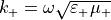 .
.
The scatterer (optical device) is contained in the lower half-space. For the sake of a simpler notation, it is assumed that the considered half-space is located above a plane with normal vector in  -direction. Hence, the plane is fully fixed by its intersection point
  with the -axis.
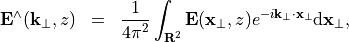
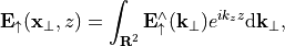
The Fourier transform of the electric field intensity with respect to  is given by
where  and
and 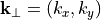 . The scaling factor in front of the integral is chosen so that the inverse Fourier transform,

reads as an infinite superposition of plane waves. The integrals are understood in a general (distributional) sense. Hence, the Fourier transform  may split into a continuous spectrum and a discrete spectrum consisting of
  -functions. This way, the periodic geometries as well as isolated geometries are treated within a common framework.
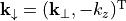
In the above, the electric field  is the total field. It is shown in the appendix to this section, that the total field allows a splitting into an upward directed part and a downward directed part,
  and
and  , respectively:
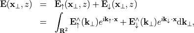
where 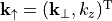 ,
,  , and with
  .
.
To discuss this splitting in greater detail, it is assumed that the material in the upper half-space is non-dissipative, so that  is a real positive number, and hence,

When  ,
,  is an upward propagating plane wave, whereas
  travels downward. For
  , is evanescent in -direction, since
  and hence
  . Again,
  has the opposite behavior: it increases exponentially in the positive -direction.
Note
JCMsolve computes the upward directed Fourier spectrum  . Its definition is independent of the -position of the plane.
From the energy conservation principle, it follows that the downward directed part only stems from the illumination. However, the illumination may also contain upward directed waves due to reflections or transmissions. Generally, the illuminating field may allow for a splitting into upward and downward directed parts:

with corresponding splitting of its Fourier transform

For example, when the scatterer is embedded into a homogeneous medium or into a layered media stack, and when illuminated by a plane wave from below,  is zero and
  is the prescribed plane wave as it leaves the multilayer stack. Then, the Fourier transform of the upward directed field can be decomposed into the scattered part and the illumination part:

For isolated structures, the Fourier transform  of the scattered field is a smooth function of
  (except a branch cut singularity at
  ). In contrast to this, the Fourier transform of the illumination is often discrete. For example, when the illumination has a transmitted or reflected plane wave in the upper half-space with k-vector
  and amplitude
  , then

The presence of a continuous and a discrete spectrum in  necessitates a proper book-keeping in the output file. This is discussed below, when detailing the output format.
Periodic geometries
See Electromagnetics for the discussion of periodic boundary conditions in the context of electromagnetic field computation. There, it is claimed that the electromagnetic field satisfies Bloch-periodic boundary conditions
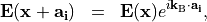
with a given Bloch vector  , and for one or more lattice vectors
  . To fit with the representation above, it is assumed that the lattice vectors are located in the
  -coordinate plane. This way, one gets for the upward propagating field:

I) Twofold periodic case:
There exist two lattice vectors  and
and  with reciprocal grid vectors
  ,
,  , such that
The function  is lattice periodic, and therefore, it allows for an expansion into discrete Fourier modes:
Warning
As a convention the lattice vectors and are ordered, so that  (
( -direction of the first lattice vector) is maximized, and , together with
  form an orthonormal coordinate system. Here, is the normal propagation direction of the scattered field, that is
 ![\pvec{n}=[0\,0\,1]](_images/math/0e0fd3c5b64f1f632e7cfdfe7afb1d0feb2db801.png) for
for NormalDirection=Z and ![\pvec{n}=[0\,0\,-1]](_images/math/74528afa61b50ba7574602c870a587d151cfd018.png) for
for NormalDirection=-Z.
with  , and
with
, and
with  as defined above.
With this, the upward propagating field can be written as an inverse Fourier transform
with
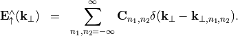
Hence the Fourier spectrum is fully discrete.
II) Onefold periodic case:
It is assumed that the single grid vector  is aligned with the -coordinate direction, i.e.,
 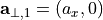 . The reciprocal lattice vector is given as
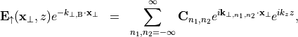
 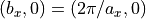 . Considerations similar to the treatment of the twofold periodic case lead to a Fourier transform of the following shape,

Hence, it is discrete in  but still a continuous spectrum in
  .
.
Storage format
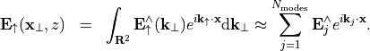
The computed Fourier transform is stored in a JCM table under the path OutputFileName. Each row in the table corresponds to a plane wave with angular wave number  stored in the first the columns. Summing up (superimposing) these plane waves gives an approximation of the upward directed field:
The output JCM table file has the following columns:
Columns 1-3: KX, KY, KZ
This is
as explained above.Columns 4-5: N1, N2
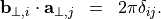
These columns are only present for geometries with a pure discrete spectrum. The integer numbers refers to the diffraction orders as defined by the reciprocal grid vectors, so that
![[k_x, k_y] = \pvec{k}_{\mathrm{B}} + n_1 \pvec{b}_{\perp, 1}+n_2 \pvec{b}_{\perp, 2}](_images/math/7c61949bc220564448bff3a9f18d211de8852b35.png) .
.Columns …: <Quantity>X_<iF>, <Quantity>Y_<iF>, <Quantity>Z_<iF>,
Here,
<Quantity>is the tag of the field quantity, e.g.,ElectricFieldStrengthorMagneticFieldStrength. The index<iF>stands for the field index. The,  , and components of one field are stored in consecutive columns.
The continuous and discrete spectra are treated in the same way. However, when the user wishes to perform an up-sampling of the computed Fourier spectrum, one must distinguish between the continuous and the discrete spectra: Only the continuous spectrum can be interpolated on a finer mesh in the  -space. The discrete spectrum is fixed. To support for this, the header of the table contains an integer entry
 NContinuousSpectrumModes, here called  . The first corresponds to an sampling of the continuous spectrum on a regular grid in the -space. Note that
  is equal to
  at up to an scaling factor proportional the the cell volume of the underlying mesh in the -space.
Appendix: Splitting into downward and upward directed waves.
It is shown how the total field can be split into an upward directed part and a downward directed part, and , respectively:

The electric field satisfies Maxwell’s equations in the upper homogeneous half-space with scalar permittivity and permeability , and with no impressed sources:
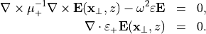
This second equation is the divergence condition. Applying this on both sides of the above equation defining the inverse Fourier transform above yields
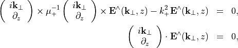
with the angular wave number 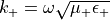 of the upper half-space.
Expanding these equations shows that each component  of the electric field satisfies the scalar equation

which permits the general solution

with .
Switching back to the vectorial Maxwell’s equations and applying the inverse Fourier transform yields the desired representation of the electric field in the upper half-space:

where and .